直方图
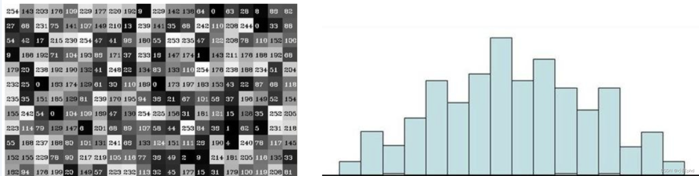
cv2.calcHist(images,channels,mask,histSize,ranges)
- images: 原图像图像格式为 uint8 或 float32。当传入函数时应 用中括号 [] 括来例如[img]
- channels: 同样用中括号括来它会告函数我们统幅图 像的直方图。如果入图像是灰度图它的值就是 [0]如果是彩色图像 的传入的参数可以是 [0][1][2] 它们分别对应着 BGR。
- mask: 掩模图像。统整幅图像的直方图就把它为 None。但是如 果你想统图像某一分的直方图的你就制作一个掩模图像并 使用它。
- histSize:BIN 的数目。也应用中括号括来
- ranges: 像素值范围常为 [0256]
import cv2 #opencv读取的格式是BGR
import numpy as np
import matplotlib.pyplot as plt#Matplotlib是RGB
def cv_show(img,name):
cv2.imshow(name,img)
cv2.waitKey()
cv2.destroyAllWindows()
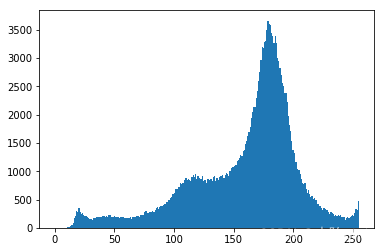
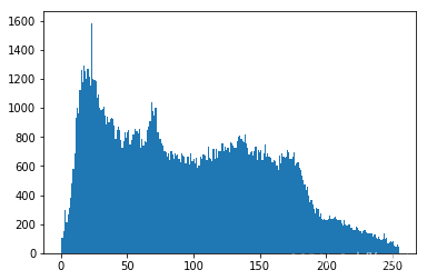
img = cv2.imread('cat.jpg',0) #0表示灰度图
hist = cv2.calcHist([img],[0],None,[256],[0,256])
hist.shape
plt.hist(img.ravel(),256);
plt.show()
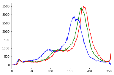
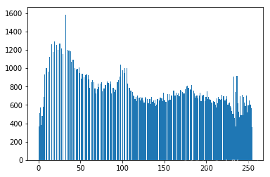
bgr三分量显示
img = cv2.imread('cat.jpg')
color = ('b','g','r')
for i,col in enumerate(color):
    histr = cv2.calcHist([img],[i],None,[256],[0,256])
    plt.plot(histr,color = col)
    plt.xlim([0,256])
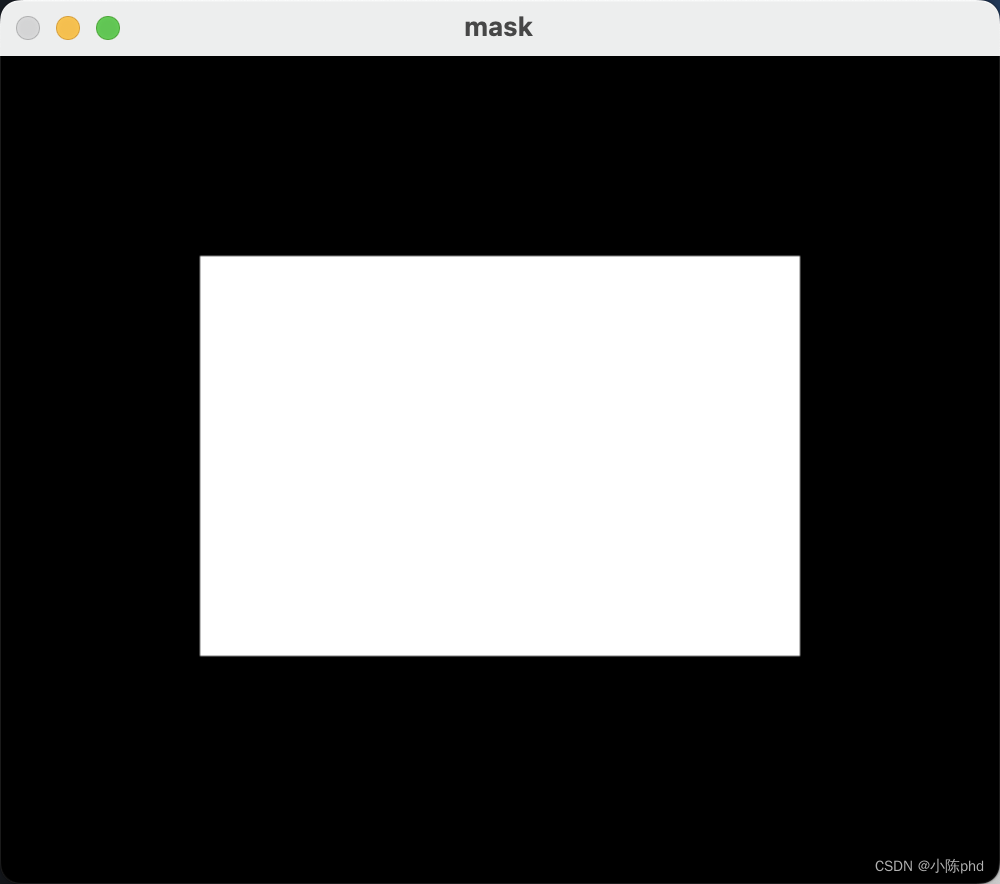
mask 操作
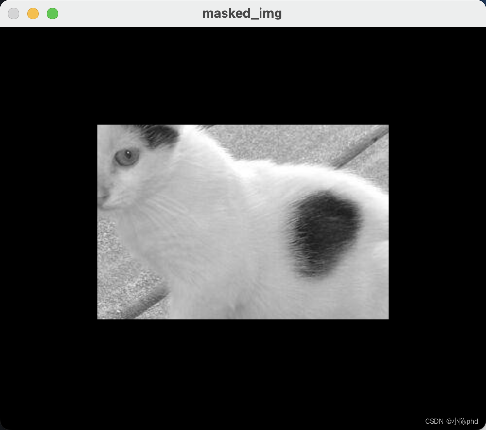
# 创建mast
mask = np.zeros(img.shape[:2], np.uint8)
print (mask.shape)
mask[100:300, 100:400] = 255
cv_show(mask,'mask')
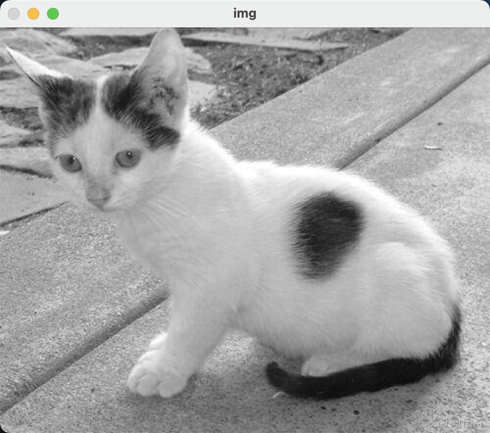
img = cv2.imread('cat.jpg', 0)
cv_show(img,'img')
masked_img = cv2.bitwise_and(img, img, mask=mask)#与操作
cv_show(masked_img,'masked_img')
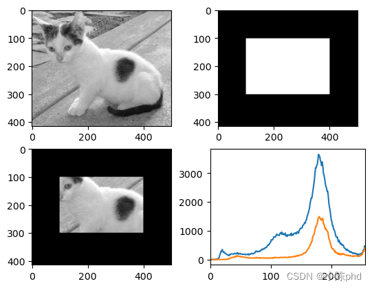
plt.subplot(221), plt.imshow(img, 'gray')
plt.subplot(222), plt.imshow(mask, 'gray')
plt.subplot(223), plt.imshow(masked_img, 'gray')
plt.subplot(224), plt.plot(hist_full), plt.plot(hist_mask)
plt.xlim([0, 256])
plt.show()
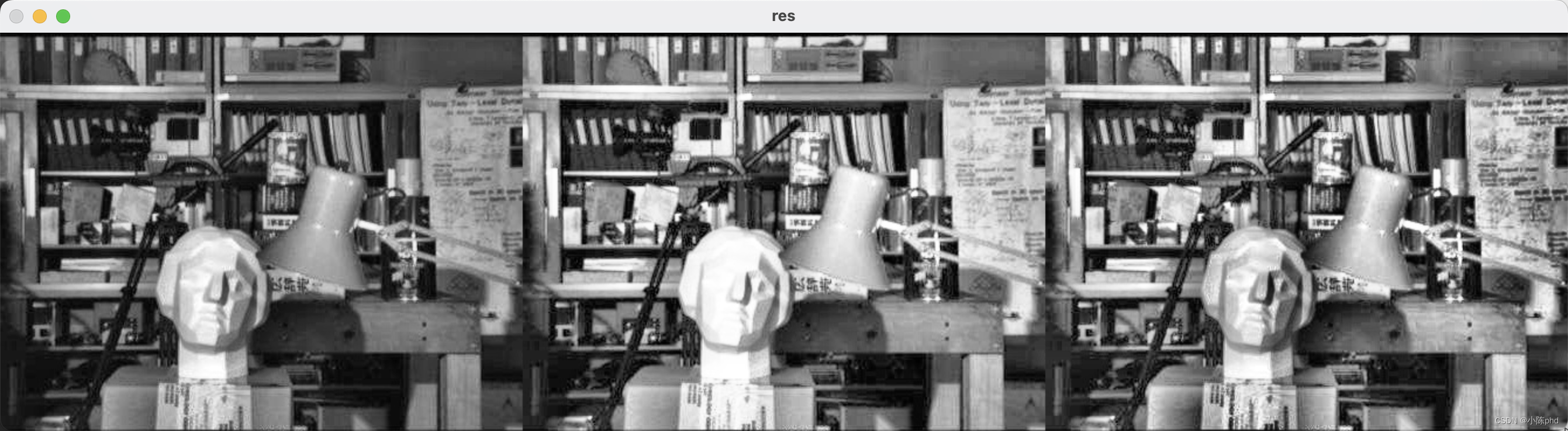
直方图均衡化
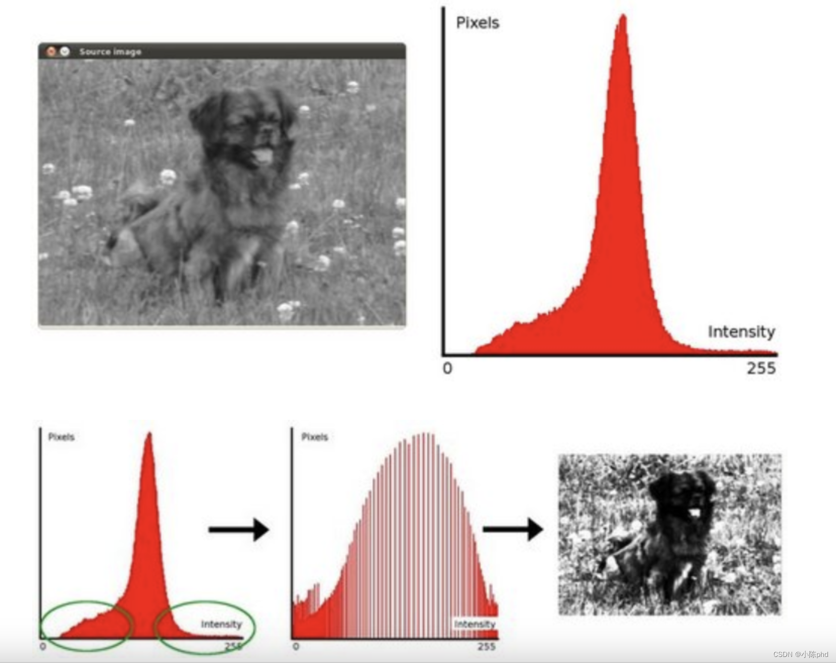
img = cv2.imread('clahe.jpg',0) #0表示灰度图 #clahe
plt.hist(img.ravel(),256);
plt.show()
equ = cv2.equalizeHist(img)
plt.hist(equ.ravel(),256)
plt.show()
自适应直方图均衡化
clahe = cv2.createCLAHE(clipLimit=2.0, tileGridSize=(8,8))
res_clahe = clahe.apply(img)
res = np.hstack((img,equ,res_clahe))
cv_show(res,'res')
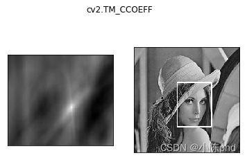
模版匹配
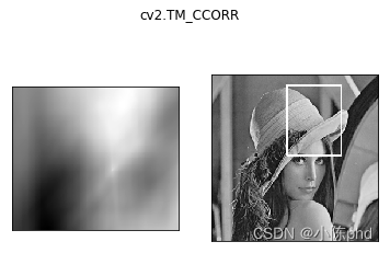
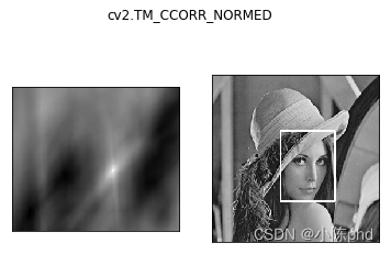
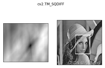
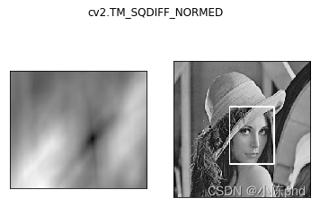
模板匹配和卷积原理很像,模板在原图像上从原点开始滑动,计算模板与(图像被模板覆盖的地方)的差别程度,这个差别程度的计算方法在opencv里有6种,然后将每次计算的结果放入一个矩阵里,作为结果输出。假如原图形是AxB大小,而模板是axb大小,则输出结果的矩阵是(A-a+1)x(B-b+1)
# 模板匹配
img = cv2.imread('lena.jpg', 0)
template = cv2.imread('face.jpg', 0)
h, w = template.shape[:2]
- TM_SQDIFF:计算平方不同,计算出来的值越小,越相关
- TM_CCORR:计算相关性,计算出来的值越大,越相关
- TM_CCOEFF:计算相关系数,计算出来的值越大,越相关
- TM_SQDIFF_NORMED:计算归一化平方不同,计算出来的值越接近0,越相关
- TM_CCORR_NORMED:计算归一化相关性,计算出来的值越接近1,越相关
- TM_CCOEFF_NORMED:计算归一化相关系数,计算出来的值越接近1,越相关
methods = ['cv2.TM_CCOEFF', 'cv2.TM_CCOEFF_NORMED', 'cv2.TM_CCORR',
           'cv2.TM_CCORR_NORMED', 'cv2.TM_SQDIFF', 'cv2.TM_SQDIFF_NORMED']
res = cv2.matchTemplate(img, template, cv2.TM_SQDIFF)
min_val, max_val, min_loc, max_loc = cv2.minMaxLoc(res)
for meth in methods:
    img2 = img.copy()

    # 匹配方法的真值
    method = eval(meth)
    print (method)
    res = cv2.matchTemplate(img, template, method)
    min_val, max_val, min_loc, max_loc = cv2.minMaxLoc(res)

    # 如果是平方差匹配TM_SQDIFF或归一化平方差匹配TM_SQDIFF_NORMED,取最小值
    if method in [cv2.TM_SQDIFF, cv2.TM_SQDIFF_NORMED]:
        top_left = min_lo   c
    else:
        top_left = max_loc
    bottom_right = (top_left[0] + w, top_left[1] + h)

    # 画矩形
    cv2.rectangle(img2, top_left, bottom_right, 255, 2)

    plt.subplot(121), plt.imshow(res, cmap='gray')
    plt.xticks([]), plt.yticks([])  # 隐藏坐标轴
    plt.subplot(122), plt.imshow(img2, cmap='gray')
    plt.xticks([]), plt.yticks([])
    plt.suptitle(meth)
    plt.show()

匹配多个对象
img_rgb = cv2.imread('mario.jpg')
img_gray = cv2.cvtColor(img_rgb, cv2.COLOR_BGR2GRAY)
template = cv2.imread('mario_coin.jpg', 0)
h, w = template.shape[:2]

res = cv2.matchTemplate(img_gray, template, cv2.TM_CCOEFF_NORMED)
threshold = 0.8
# 取匹配程度大于%80的坐标
loc = np.where(res >= threshold)
for pt in zip(*loc[::-1]):  # *号表示可选参数
    bottom_right = (pt[0] + w, pt[1] + h)
    cv2.rectangle(img_rgb, pt, bottom_right, (0, 0, 255), 2)

cv2.imshow('img_rgb', img_rgb)
cv2.waitKey(0)