Analytic-Splatting: Anti-Aliased 3D Gaussian Splatting via Analytic Integration
解析溅射:通过解析积分进行抗混叠的3D高斯溅射
Abstract 摘要 Analytic-Splatting: Anti-Aliased 3D Gaussian Splatting via Analytic Integration
The 3D Gaussian Splatting (3DGS) gained its popularity recently by combining the advantages of both primitive-based and volumetric 3D representations, resulting in improved quality and efficiency for 3D scene rendering. However, 3DGS is not alias-free, and its rendering at varying resolutions could produce severe blurring or jaggies. This is because 3DGS treats each pixel as an isolated, single point rather than as an area, causing insensitivity to changes in the footprints of pixels. Consequently, this discrete sampling scheme inevitably results in aliasing, owing to the restricted sampling bandwidth. In this paper, we derive an analytical solution to address this issue. More specifically, we use a conditioned logistic function as the analytic approximation of the cumulative distribution function (CDF) in a one-dimensional Gaussian signal and calculate the Gaussian integral by subtracting the CDFs. We then introduce this approximation in the two-dimensional pixel shading, and present Analytic-Splatting, which analytically approximates the Gaussian integral within the 2D-pixel window area to better capture the intensity response of each pixel. Moreover, we use the approximated response of the pixel window integral area to participate in the transmittance calculation of volume rendering, making Analytic-Splatting sensitive to the changes in pixel footprint at different resolutions. Experiments on various datasets validate that our approach has better anti-aliasing capability that gives more details and better fidelity.
3D高斯溅射(3DGS)结合了连续和体3D表示的优点,提高了3D场景绘制的质量和效率。然而,3DGS不是无锯齿的,它在不同分辨率下的渲染可能会产生严重的模糊或锯齿。这是因为3DGS将每个像素视为孤立的单个点而不是区域,从而导致对像素轮廓线的变化不敏感。因此,由于有限的采样带宽,这种离散采样方案不可避免地导致混叠。在本文中,我们推导出一个解析解来解决这个问题。更具体地说,我们使用条件逻辑函数作为一维高斯信号中的累积分布函数(CDF)的解析近似,并通过减去CDF来计算高斯积分。 然后,我们在二维像素着色中引入这种近似,并提出了解析溅射,它解析地近似2D像素窗口区域内的高斯积分,以更好地捕获每个像素的强度响应。此外,我们使用像素窗口积分面积的近似响应来参与体绘制的透射率计算,使得Analytic-Splatting对不同分辨率下像素足迹的变化敏感。在不同数据集上的实验表明,该方法具有更好的抗锯齿能力,提供了更多的细节和更好的保真度。
Keywords:
3D Gaussian Splatting Anti-Aliasing View Synthesis Cumulative Distribution Function (CDF) Analytic Approximation关键词:3D高斯溅射抗混叠视图合成累积分布函数解析逼近
1Work was done during an internship at Tencent AI Lab.
工作是在腾讯AI Lab实习期间完成的。2Corresponding authors. 通讯作者。

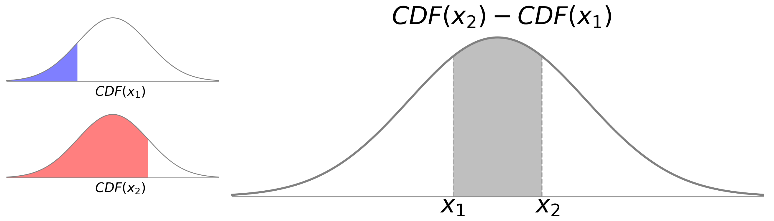
Figure 1:For shading a pixel by a Gaussian signal, 3DGS (a) only treats the Gaussian signal value corresponding to the pixel center as the intensity response. Analytic-Splatting (b) instead considers an analytic approximation of the integral over the pixel window area as the intensity response. Compared to 3DGS, Analytic-Splatting has anti-aliasing capability and better detail fidelity.
图1:为了通过高斯信号对像素进行着色,3DGS(a)仅将对应于像素中心的高斯信号值视为强度响应。解析溅射(B)替代地将像素窗口区域上的积分的解析近似视为强度响应。与3DGS相比,分析飞溅具有抗锯齿能力和更好的细节保真度。
1Introduction 一、导言
Novel view synthesis of a scene captured from multiple images has achieved great progress due to the rapid advancements of neural rendering. As a prominent representative, Neural Radiance Field (NeRF) [23] models the scene using a neural volumetric representation, enabling photorealistic rendering of novel views via ray marching. Ray marching trades off rendering efficiency with quality, and subsequent works [33, 8, 24] are proposed to have a better quality-efficiency balance. More recently, 3D Gaussian Splatting (3DGS) [16] proposes a GPU-friendly differentiable rasterization pipeline that incorporates an explicit point-based representation, achieving high-quality and real-time renderings for novel view synthesis. In contrast to ray marching in NeRF, which renders a pixel by accumulating the radiance of samples along the ray that intersects the image plane at the pixel, 3DGS employs a forward-mapping technique that can be rasterized very efficiently. Specifically, 3DGS represents the scene as a set of anisotropic 3D Gaussians with scene properties; when rendering a pixel, 3DGS orders and projects these 3D Gaussians onto the image plane as 2D Gaussians, and then queries values and scene properties associated with the Gaussians that have overlaps with the pixel, and finally shades the pixel by cumulatively compositing these queried values and properties.
由于神经绘制技术的快速发展,从多幅图像中获取场景的视图合成已经取得了很大的进展。作为一个突出的代表,神经辐射场(NeRF)[ 23]使用神经体积表示对场景进行建模,通过光线行进实现新颖视图的照片级真实感渲染。光线行进在渲染效率与质量之间进行权衡,并且随后的作品[ 33,8,24]被提议具有更好的质量-效率平衡。最近,3D高斯溅射(3DGS)[ 16]提出了一种GPU友好的可微分光栅化流水线,该流水线包含显式的基于点的表示,实现了高质量和实时渲染,用于新颖的视图合成。与NeRF中的光线行进(其通过沿着在像素处与图像平面相交的光线沿着累积样本的辐射率来渲染像素)相比,3DGS采用可以非常有效地光栅化的前向映射技术。 具体地,3DGS将场景表示为具有场景属性的各向异性3D高斯的集合;当渲染像素时,3DGS将这些3D高斯排序并投影到图像平面上作为2D高斯,然后查询与像素重叠的高斯相关联的值和场景属性,最后通过累积合成这些查询的值和属性来对像素进行着色。
3DGS works for scene representation learning and novel view synthesis at constant resolutions; however, its performance degrades greatly either when the multi-view images are captured at varying distances, or when the novel view to be rendered has a resolution different from those of the captured images. The main reason is that the footprint
3DGS适用于场景表示学习和恒定分辨率下的新视图合成;然而,当在不同距离处捕获多视图图像时,或者当要渲染的新视图具有与捕获图像不同的分辨率时,其性能大大降低。主要原因是,11The footprint is defined as the ratio between the pixel window area in screen space and its covered Gaussian signals region in the world space.
覆盖区定义为屏幕空间中的像素窗口面积与其在世界空间中覆盖的高斯信号区域之间的比率。 of the pixel changes at different resolutions and 3DGS is insensitive to such changes since it treats each pixel as an isolated point (i.e. merely pixel center) when retrieving the corresponding Gaussian values; Fig. 1a gives an illustration. As a result, 3DGS could produce significant artifacts (e.g. blurry or jaggies) especially when pixel footprints change drastically (e.g. synthesizing novel views with zooming-in and zooming-out effects).
在不同分辨率下像素的变化,3DGS对这种变化不敏感,因为它在检索相应的高斯值时将每个像素视为孤立点(即仅仅是像素中心);图1a给出了说明。因此,3DGS可能会产生明显的伪影(例如模糊或锯齿状),特别是当像素足迹急剧变化时(例如合成具有放大和缩小效果的新视图)。
By delving into the details, we know that 3DGS represents a continuous signal in the image space as a set of �-blended 2D Gaussians, and the pixel shading is a process of integrating the signal response within each pixel area; artifacts in 3DGS are caused by the limited sampling bandwidth for the Gaussians that retrieves erroneous responses, especially when the pixel footprint changes drastically. It is possible to increase sampling bandwidth (i.e. via super sampling) or use prefiltering techniques to alleviate this problem; for example, Mip-Splatting [36] employs the prefiltering technique and presents a hybrid filtering mechanism to regularize the high-frequency components of 2D and 3D Gaussians to achieve anti-aliasing. While Mip-Splatting overcomes most aliasing in 3DGS, it is limited in capturing details and synthesizes over-smoothing results. Consequently, solving the integral of Gaussian signals within the pixel window area as intensity responses is crucial for both anti-aliasing and capturing details.
通过深入研究细节,我们知道3DGS将图像空间中的连续信号表示为一组 � 混合的2D高斯,并且像素着色是在每个像素区域内整合信号响应的过程; 3DGS中的伪影是由高斯的有限采样带宽引起的,该高斯检索错误的响应,特别是当像素足迹急剧变化时。可以增加采样带宽(即通过超采样)或使用预滤波技术来缓解这个问题;例如,Mip-Splatting [ 36]采用预滤波技术并提出混合滤波机制来正则化2D和3D高斯的高频分量以实现抗混叠。虽然Mip-Splatting克服了3DGS中的大多数锯齿,但它在捕捉细节和合成过度平滑结果方面受到限制。 因此,求解像素窗口区域内高斯信号的积分作为强度响应对于抗混叠和捕获细节都是至关重要的。
In this paper, we revisit pixel shading in 3DGS and introduce an analytic approximation of the window integral response of Gaussian signals for anti-aliasing. Rather than discrete sampling in 3DGS and prefiltering in Mip-Splatting, we analytically approximate the integral within each pixel area as shown in Fig. 1b. We term our method as Analytic-Splatting. Compared with Mip-Splatting, which approximates the pixel window as a 2D Gaussian low-pass filter, our proposed method does not suppress the high-frequency components in Gaussian signals and can better preserve high-quality details. Experiments show that our method removes the aliasing existing in 3DGS and other methods while synthesizing more details with better fidelity. We summarize our contributions as follows.
在本文中,我们重新审视3DGS中的像素着色,并介绍了一个解析近似的窗口积分响应的高斯信号抗混叠。与3DGS中的离散采样和Mip—Splatting中的预滤波不同,我们解析地近似每个像素区域内的积分,如图1b所示。我们称我们的方法为分析飞溅。与将像素窗口近似为二维高斯低通滤波器的Mip—Splatting相比,该方法不抑制高斯信号中的高频成分,能更好地保留高质量的细节。实验结果表明,该方法在消除3DGS和其他方法中存在的混叠的同时,合成了更多的细节,具有更好的保真度。我们将我们的贡献总结如下。
- •
We revisit the causes of aliasing in 3D Gaussian Splatting from the perspective of signal window response and derive an analytic approximation of the window response for Gaussian signals;
·我们从信号窗口响应的角度重新审视了3D高斯溅射中混叠的原因,并推导出高斯信号的窗口响应的解析近似; - •
Based on the derivation, we present Analytic-Splatting that improves the pixel shading in 3D Gaussian Splatting to achieve anti-aliasing and better detail fidelity.
·在此基础上,我们提出了一种改进3D高斯溅射像素着色的解析溅射算法,以实现抗锯齿和更好的细节保真度。 - •
Our experiments on challenging datasets demonstrate the superiority of our method to other approaches in terms of anti-aliasing and synthesizing results.
·我们在具有挑战性的数据集上的实验证明了我们的方法在抗锯齿和合成结果方面优于其他方法。
2Related Works 2相关作品
Neural Rendering. Recently, neural rendering techniques exemplified by Neural Radiance Field (NeRF) [23] have achieved impressive results in novel view synthesis, and further enhanced several advanced tasks [30, 34, 21, 14, 22, 25]. Nevertheless, the backward-mapping volume rendering used in NeRF hinders the real-time rendering performance, restricting the application prospects of NeRF. While several NeRF variants adopt efficient sampling strategies [35, 24, 19] or use explicit/hybrid representations [8, 29, 5, 9] with higher capacities, they still suffer from the tough sampling problem and struggle with real-time rendering. To overcome these limitations, 3DGS [16] employs forward mapping volume rendering technology and implements GPU-friendly tile-based rasterization to achieve real-time rendering and impressive rendering results. Due to its real-time rendering capability and impressive rendering performance, 3DGS has been widely used in advanced tasks such as Human/Avatar modeling [27, 12, 38, 40], surface reconstruction [10, 6], inverse rendering [20, 15, 28], physical simulation [32, 7], etc. Although rasterization makes 3DGS avoid tough sampling problems along rays and achieve promising results, it also introduces aliasing caused by restricted sampling bandwidth when shading pixels using 2D Gaussians. And the aliasing will be noticeable when the pixel footprint changes drastically (e.g. zooming in and out). In this paper, we study the errors introduced by the discrete sampling scheme used in 3DGS and introduce our advanced resolution.
神经渲染。最近,以神经辐射场(NeRF)[ 23]为例的神经渲染技术在新颖的视图合成中取得了令人印象深刻的结果,并进一步增强了几个高级任务[ 30,34,21,14,22,25]。然而,NeRF中采用的后向映射体绘制方法阻碍了实时绘制性能,限制了NeRF的应用前景。虽然几个NeRF变体采用了有效的采样策略[ 35,24,19]或使用具有更高容量的显式/混合表示[ 8,29,5,9],但它们仍然存在坚韧的采样问题,并且难以实时渲染。为了克服这些限制,3DGS [ 16]采用前向映射体绘制技术,并实现GPU友好的基于瓦片的光栅化,以实现实时渲染和令人印象深刻的渲染结果。 由于其实时渲染能力和令人印象深刻的渲染性能,3DGS已被广泛用于高级任务,如人类/化身建模[ 27,12,38,40],表面重建[ 10,6],逆渲染[ 20,15,28],物理模拟[ 32,7],虽然光栅化使得3DGS避免了沿沿着射线的坚韧采样问题并获得了有希望的结果,但是当使用2D高斯对像素进行着色时,光栅化也引入了由有限的采样带宽引起的混叠。当像素占用空间急剧变化时(例如放大和缩小),混叠将是明显的。在本文中,我们研究了3DGS中使用的离散采样方案所引入的误差,并介绍了我们的先进的解决方案。
Anti-Aliasing. Aliasing is the phenomenon of overlapping frequency components when the discrete sampling rate is below the Nyquist rate. Anti-aliasing is critical for rendering high-fidelity results, which has been extensively explored in the computer graphics and vision community [1, 31, 18]. In the neural rendering context, MipNeRF [2] and Zip-NeRF [4] pioneer the use of prefiltering and multi-sampling to address the aliasing issue in neural radiance fields (NeRF). Recent works also explored the anti-aliased NeRF for unbounded scenes [3], efficient reconstruction [13], and surface reconstruction [39]. All these works are built upon the backward-mapping volume rendering to consider the pixel footprint, by replacing the original ray-casting with cone-casting. However, the backward-mapping volume rendering is too computationally expensive to achieve real-time rendering. On the other hand, 3DGS [16] introduced real-time forward-mapping volume rendering but suffers from aliasing artifacts due to the discrete sampling during shading pixels using projected Gaussians. To this end, Mip-Splatting [36] presents a hybrid filtering mechanism to restrict the high-frequency components of 2D and 3D Gaussians to achieve anti-aliasing. Nevertheless, this low-pass filtering strategy hinders the capability to preserve high-quality details. In contrast, our approach introduces an analytic approximation of the integral within the pixel area to better capture the intensity response of each pixel, harvesting both aliasing-free and detail-preserving rendering results.
抗锯齿。混叠是当离散采样率低于奈奎斯特速率时频率分量重叠的现象。抗锯齿对于渲染高保真结果至关重要,这在计算机图形和视觉社区中得到了广泛的探索[ 1,31,18]。在神经渲染上下文中,MipNeRF [ 2]和Zip-NeRF [ 4]率先使用预滤波和多采样来解决神经辐射场(NeRF)中的混叠问题。最近的工作还探索了无界场景的抗锯齿NeRF [ 3],有效重建[ 13]和表面重建[ 39]。所有这些工作都是建立在向后映射体绘制考虑像素足迹,取代原来的光线投射与锥投射。然而,向后映射体绘制的计算量太大,无法实现实时绘制。 另一方面,3DGS [16]引入了实时前向映射体绘制,但由于使用投影高斯对像素进行着色期间的离散采样而遭受混叠伪影。为此,Mip—Splatting [36]提出了一种混合滤波机制,以限制2D和3D高斯的高频分量,从而实现抗混叠。然而,这种低通滤波策略阻碍了保持高质量细节的能力。相比之下,我们的方法引入了像素区域内积分的解析近似,以更好地捕获每个像素的强度响应,从而获得无混叠和细节保留的渲染结果。
3Preliminary 3初步
In this section, we give the technical background necessary for presentation of our proposed method.
在本节中,我们给予介绍我们提出的方法所需的技术背景。
3D Gaussian Splatting (3DGS) explicitly represents 3D scene as a set of points {𝒑�}�=1�. Given any point 𝒑∈{𝒑�}�=1�, 3DGS models it as a 3D Gaussian signal with mean vector 𝝁 and covariance matrix 𝚺:
3D高斯溅射(3DGS)将3D场景明确表示为点 {𝒑�}�=1� 的集合。给定任何点 𝒑∈{𝒑�}�=1� ,3DGS将其建模为具有均值向量 𝝁 和协方差矩阵 𝚺 的3D高斯信号:
| �3D(𝒙|𝝁,𝚺)=exp(−12(𝒙−𝝁)⊤𝚺−1(𝒙−𝝁)), | (1) |
where 𝝁∈ℝ3 is the position of point 𝒑, and 𝚺∈ℝ3×3 is an anisotropic covariance matrix, which is factorized into a scaling matrix 𝑺 and a rotation matrix 𝑹 as 𝚺=𝑹𝑺𝑺⊤𝑹⊤. Note that 𝑺 indicates a 3×3 diagonal matrix and 𝑹 refers to a 3×3 matrix constructed from a unit quaternion 𝒒.
其中 𝝁∈ℝ3 是点 𝒑 的位置,并且 𝚺∈ℝ3×3 是各向异性协方差矩阵,其被分解为缩放矩阵 𝑺 和旋转矩阵 𝑹 作为 𝚺=𝑹𝑺𝑺⊤𝑹⊤ 。注意, 𝑺 指示 3×3 对角矩阵,并且 𝑹 指的是从单位四元数 𝒒 构造的 3×3 矩阵。
Given a viewing transformation with extrinsic matrix 𝑻 and projection matrix 𝑲, we get the projected position 𝝁^ and covariance matrix 𝚺^ in 2D screen space as:
给定具有外部矩阵 𝑻 和投影矩阵 𝑲 的观看变换,我们得到2D屏幕空间中的投影位置 𝝁^ 和协方差矩阵 𝚺^ 为:
| 𝝁^=𝑲𝑻[𝝁,1]⊤,𝚺^=𝑱𝑻𝚺𝑻⊤𝑱⊤, | (2) |
where 𝑱 is the Jacobian matrix of the affine approximation of the perspective projection. Note that 3DGS only retains the second-order values of 𝝁^ and 𝚺^ as 𝝁^∈ℝ2 and 𝚺^∈ℝ2×2 respectively. The projected 2D Gaussian signal for the pixel 𝒖 is given:
其中 𝑱 是透视投影的仿射近似的雅可比矩阵。注意,3DGS仅将 𝝁^ 和 𝚺^ 的二阶值分别保留为 𝝁^∈ℝ2 和 𝚺^∈ℝ2×2 。给出像素 𝒖 的投影2D高斯信号:
| �2D(𝒖|𝝁^,𝚺^)=exp(−12(𝒖−𝝁^)⊤𝚺^−1(𝒖−𝝁^)), | (3) |
using the projected 2D Gaussian signal, 3DGS derives the volume transmittance and shades the color of pixel 𝒖 through:
使用投影的2D高斯信号,3DGS通过以下步骤导出体积透射率并对像素 𝒖 的颜色进行着色:
| 𝑪(𝒖)=∑�∈�����2D(𝒖|𝝁�^,𝚺�^)��𝒄�,��=∏�=1�−1(1−��2D(𝒖|𝝁�^,𝚺�^)��), | (4) |
where the symbols with subscripts � indicate the attributes related to the point 𝒑�. Specifically, �� and 𝒄� respectively denote the opacity and view-dependent color of point 𝒑�.
其中带有下标 � 的符号表示与点 𝒑� 相关的属性。具体地, �� 和 𝒄� 分别表示点 𝒑� 的不透明度和视图相关颜色。
For better understanding, we further formulate the 2D Gaussian signal �2D in Eq. 3 as a flattened expression. Considering 𝚺^ is a real-symmetric 2×2 matrix, we numerically express 𝚺^ and 𝚺^−1 as:
为了更好地理解,我们进一步在等式(1)中用公式表示2D高斯信号 �2D 。3、一个简单的表达考虑到 𝚺^ 是实对称的 2×2 矩阵,我们将 𝚺^ 和 𝚺^−1 数值表示为:
| 𝚺^=[Σ^11Σ^12Σ^12Σ^22] | ,𝚺^−1=1|𝚺^|[Σ^22−Σ^12−Σ^12Σ^11]=[����], | (5) | ||
| � | =Σ^22|𝚺^|,�=−Σ^12|𝚺^|,�=Σ^11|𝚺^|, |
given the pixel 𝒖=[��,��]⊤ and the projected position 𝝁^=[�^�,�^�]⊤ in 2D screen space, Eq. 3 can be rewrited as:
给定2D屏幕空间中的像素 𝒖=[��,��]⊤ 和投影位置 𝝁^=[�^�,�^�]⊤ ,等式(1)3可以改写为:
| �2D(𝒖 | |𝝁^,𝚺^)=exp(−�2�^�2−�2�^�2−��^��^�), | (6) | ||
| �^� | =��−�^�,�^�=��−�^�. |
Remark. It is worth noting that 3DGS treats each pixel as an isolated, single point when calculating its corresponding Gaussian value, as shown in Eq. (6). This approximating scheme functions effectively when training and testing images to capture the scene content from a relatively consistent distance. However, when the pixel footprint changes due to focal length or camera distance adjustments, 3DGS renderings exhibit considerable artifacts, such as thin Gaussians observed during zooming in. As a result, it becomes crucial to define the pixel as a window area and calculate the corresponding intensity response by integrating the Gaussian signal within this domain. Rather than using the intuitive but time-consuming super sampling, it would be better to tackle the problem more analytically, given that the Gaussian Signal is a continuous function.
备注。值得注意的是,3DGS在计算其对应的高斯值时将每个像素视为孤立的单个点,如等式(1)所示。(6).当训练和测试图像以从相对一致的距离捕获场景内容时,这种近似方案有效地起作用。然而,当像素覆盖区由于焦距或相机距离调整而改变时,3DGS渲染会表现出相当多的伪影,例如在放大期间观察到的薄高斯。因此,将像素定义为窗口区域并通过在该域内积分高斯信号来计算相应的强度响应变得至关重要。考虑到高斯信号是一个连续函数,与其使用直观但耗时的超采样,不如更好地分析解决这个问题。
4Methods 4方法
In Sec. 3, we observe that 3DGS ignores the window area of each pixel, and only considers the Gaussian value corresponding to the pixel center as its intensity response. This approach would inevitably produce artifacts due to fluctuations of the pixel footprint under different resolutions. To address this problem, we are motivated to derive an analytical approximation of a 2D Gaussian signal within the pixel window area to accurately describe the intensity response of the imaging pixel. Subsequently, we plan to apply this derived integration to replace �2D in the 3DGS framework.
节中3、我们观察到3DGS忽略了每个像素的窗口面积,只考虑像素中心对应的高斯值作为其强度响应。这种方法将不可避免地产生由于在不同分辨率下的像素足迹的波动的伪影。为了解决这个问题,我们的动机是推导出一个2D高斯信号的像素窗口区域内的解析近似,以准确地描述成像像素的强度响应。随后,我们计划应用此派生集成来替换3DGS框架中的 �2D 。
(a)Integration (Ground-truth)
(a)地面实况(Ground-truth)
(b)Baseline (3DGS) (b)基线(3DGS)
(c)Super Sampling (3DGS-SS)
(c)超采样(3DGS-SS)
(d)Filtering (Mip-Splatting)
(d)过滤(Mip-Splatting)
(e)Analytic Approximation (Ours)
(e)解析近似(我们的)
Figure 2:Example diagram of the signal integration within window area and the approximation schemes used in different methods.
图2:窗口区域内的信号积分示例图和不同方法中使用的近似方案。
4.1Revisit One-dimensional Gaussian Signal Response
4.1再论一维高斯信号响应
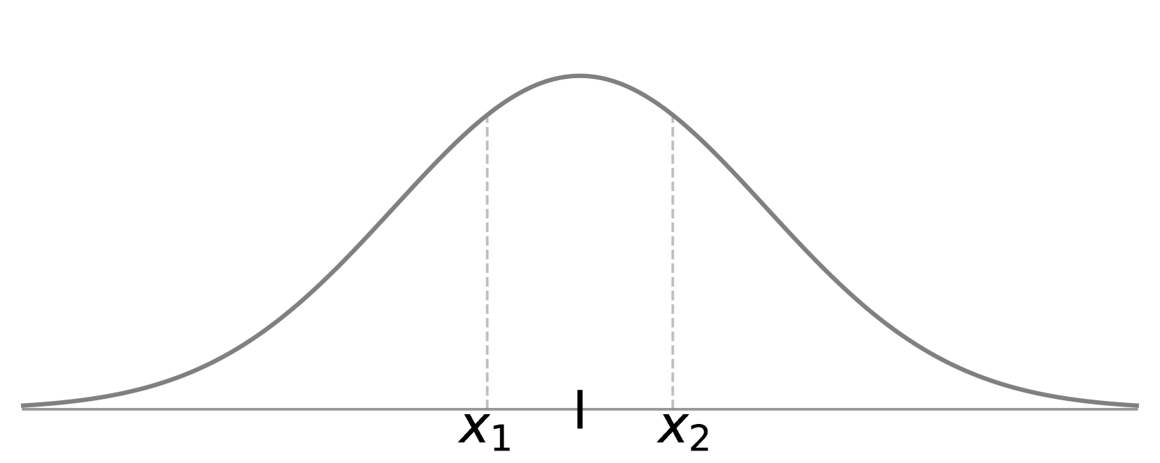
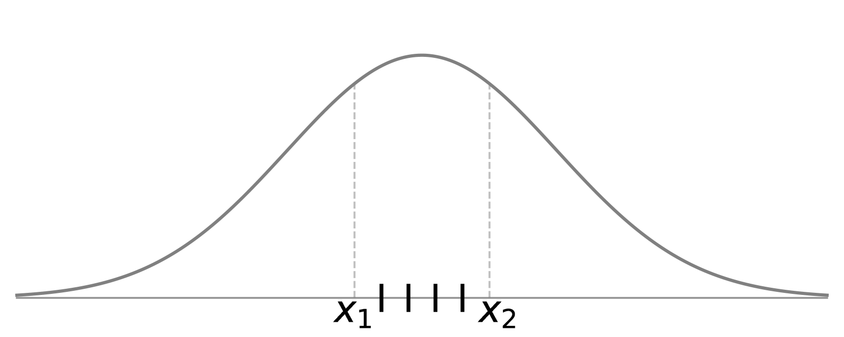
Before describing our proposed method, we first revisit the example of the integrated response of a one-dimensional Gaussian Signal within a window area for better understanding. Given a signal �(�) and a window area [�1,�2], we aim to get the response by integrating the signal ℐ�=∫�1�2�(�)d� within this domain as shown in Fig. 1(a). For an unknown signal, Monte Carlo sampling within the window area is a feasible approach to approximate the integral as demonstrated in Fig. 1(b) and Fig. 1(c), and the approximation result ℐ�≈�2−�1�∑�=1��(��),��∈[�1,�2] will be more accurate as the number of samples � increases. Nonetheless, increasing the number of samples (i.e., super sampling) increases the computation burden significantly.
在描述我们提出的方法之前,我们首先回顾一下窗口区域内一维高斯信号的积分响应的例子,以便更好地理解。给定信号 �(�) 和窗口区域 [�1,�2] ,我们的目标是通过在该域内积分信号 ℐ�=∫�1�2�(�)d� 来获得响应,如图1(a)所示。对于未知信号,在窗口区域内进行蒙特卡罗采样是一种可行的方法来近似积分,如图1(b)和图1(c)所示,并且随着样本 � 数量的增加,近似结果 ℐ�≈�2−�1�∑�=1��(��),��∈[�1,�2] 将更加准确。尽管如此,增加样本的数量(即,超采样)显著增加了计算负担。
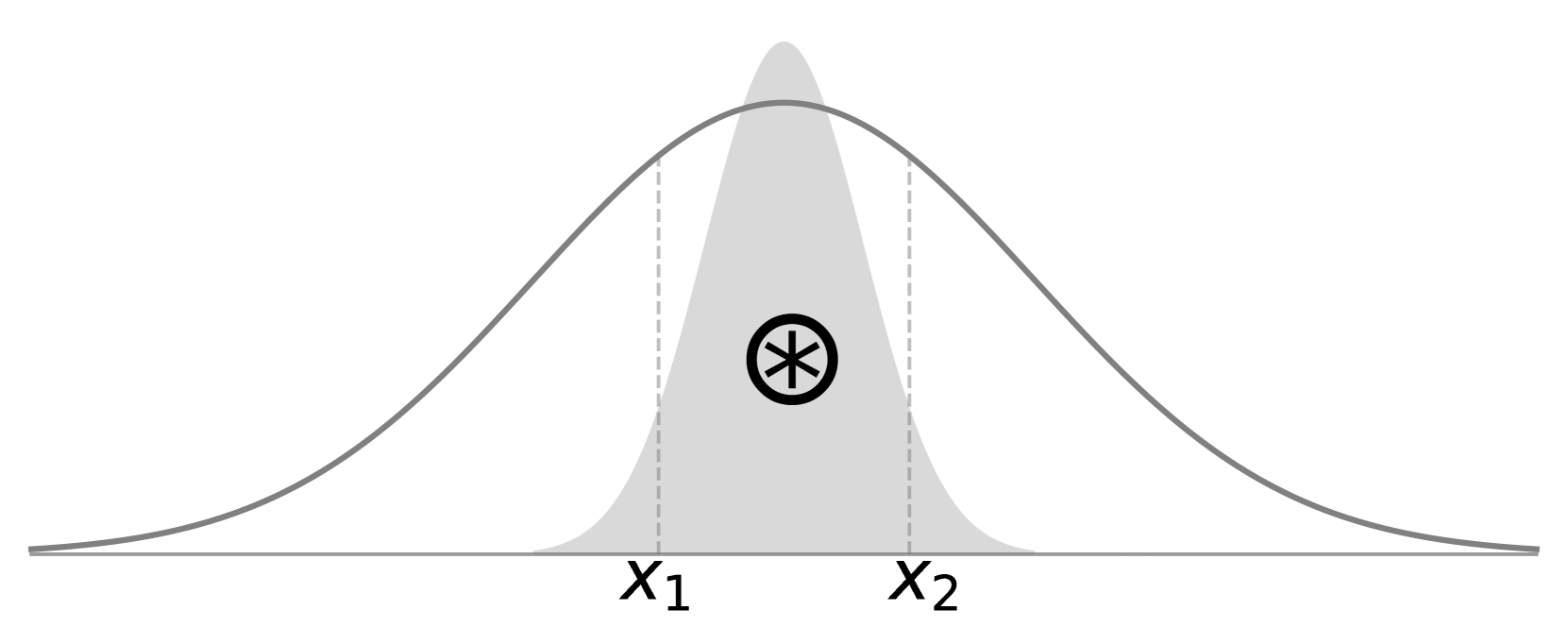
Fortunately, our goal in the 3DGS framework is to obtain the intensity response of the Gaussian signal within the window area [�1,�2]. Given that the Gaussian signal is a continuous real-valued function, it is natural to derive an analytical approximation to the Gaussian definite integral (Fig. 1(a)) which is more accurate compared to the numerical integration (Fig. 1(b) and Fig. 1(c)). For instance, in Mip-Splatting, the window area is treated as a Gaussian kernel �w, and the integral is approximated as the result of sampling after convolving the Gaussian signal with the Gaussian kernel ℐ�≈�⊛�w 22the standard deviation � in �w is set to 0.1. Note that the result of convolving a Gaussian signal with a Gaussian kernel is still a Gaussian signal
�w 中的标准偏差 � 被设置为 0.1 。注意,将高斯信号与高斯核卷积的结果仍然是高斯信号
幸运的是,我们在3DGS框架中的目标是获得窗口区域 [�1,�2] 内高斯信号的强度响应。假设高斯信号是连续实值函数,自然可以推导出高斯定积分的解析近似(图1(a)),与数值积分(图1(B)和图1(c))相比,该解析近似更精确。例如,在Mip-Splatting中,窗口区域被视为高斯核 �w ,并且积分被近似为在将高斯信号与高斯核 ℐ�≈�⊛�w 2 卷积之后的采样结果。 as shown in Fig. 1(d). While this prefiltering uses the great convolution properties of Gaussian signals, this approximation will introduce a large gap when the Gaussian signal � mainly consists of high-frequency components (i.e., with small standard variation �).
如图1(d)所示。虽然这种预滤波使用高斯信号的大卷积特性,但是当高斯信号 � 主要由高频分量组成时,这种近似将引入大的间隙(即,具有小的标准变化 � )。
To overcome these shortcomings, we are motivated to calculate the integral within the window area analytically. Specifically, the problem of evaluating the definite integral within [�1,�2] can be simplified to the subtraction of two improper integrals by applying the first part of the fundamental theorem of calculus. Let �(�) be the cumulative distribution function (CDF) of the standard Gaussian distribution �(�) defined by,
为了克服这些缺点,我们的动机是计算窗口区域内的积分解析。具体地说,利用微积分基本定理的第一部分,可以将求 [�1,�2] 内定积分的问题简化为两个广义积分的减法。令 �(�) 为标准高斯分布 �(�) 的累积分布函数(CDF),
| �(�)=∫−∞��(�)d�,�(�) | =12�exp(−�22), | (7) |
and the definite integral of �(�) within [�1,�2] can be expressed as,
并且 �(�) 在 [�1,�2] 内的定积分可以表示为,
| ℐ�=�(�2)−�(�1). | (8) |
However, this CDF of the Gaussian function (defined as the error function erf) is not closed-form. We start by approximating the CDF �(�) and find an important corollary, i.e.,
然而,高斯函数(定义为误差函数erf)的该CDF不是封闭形式的。我们从近似CDF �(�) 开始,并发现一个重要的推论,即,
Definition 1 定义1
The logistic function �(�) is the analytic approximation of the CDF �(�) with standard deviation �=1, which is defined as,
逻辑函数 �(�) 是具有标准差 �=1 的CDF �(�) 的解析近似,其被定义为,
| �(�)=11+exp(−1.6⋅�−0.07⋅�3), | (9) |
and could be derivative-friendly.
并且可以是衍生友好的。
This analytic approximation also contains similar properties of the CDF �(�):
该解析近似也包含CDF �(�) 的类似性质:
- 1.
�(�) is non-decreasing and right-continuous, satisfying
lim�→−∞�(�)=lim�→−∞�(�)=0andlim�→+∞�(�)=lim�→+∞�(�)=1.
1. �(�) 是非递减且右连续的,满足 - 2.
The curve of �(�) has 2-fold rotational symmetry around the point (0,1/2),
�(�)+�(−�)=�(�)+�(−�)=1,∀�∈ℝ.
2. 0#的曲线围绕点1#具有二重旋转对称性,
For any Gaussian signals with different standard deviations, we can approximate their CDFs by scaling � in Eq. 9 by the reciprocals of their standard deviations. Once � in �(�) scales by the reciprocal of �, we express it as ��(�). For more details, please refer to the supplementary material.
对于具有不同标准偏差的任何高斯信号,我们可以通过在等式中缩放 � 来近似它们的CDF。9的标准差的倒数。一旦 �(�) 中的 � 按 � 的倒数缩放,我们将其表示为 ��(�) 。详情请参阅补充材料。
In summary, given the sample � and setting the window area as 1, the integral ℐ�(�) of Gaussian signal �(�) within the area [�−12,�+12] is defined as:
总之,给定样本 � 并将窗口区域设置为 1 ,高斯信号 �(�) 在区域 [�−12,�+12] 内的积分 ℐ�(�) 被定义为:
| ℐ�(�)=∫�−12�+12�(�)d�=�(�+12)−�(�−12). | (10) |
Besides, according to Eq. 9, we apply Eq. 9 and approximate the integral of Eq. 10 as:
此外,根据EQ。9,我们使用Eq。9和近似的积分方程。10如:
| ℐ�(�)≈�(�+12)−�(�−12). | (11) |
In the following section, we will discuss how to employ the above approximation to 2D-pixel shading in Analytic-Splatting.
在下面的部分中,我们将讨论如何在分析飞溅中将上述近似应用于2D像素着色。

(a)Integral over the original pixel area.
(a)在原始像素区域上积分。

(b)Integral over the rotated pixel area.
(b)旋转像素区域上的积分。
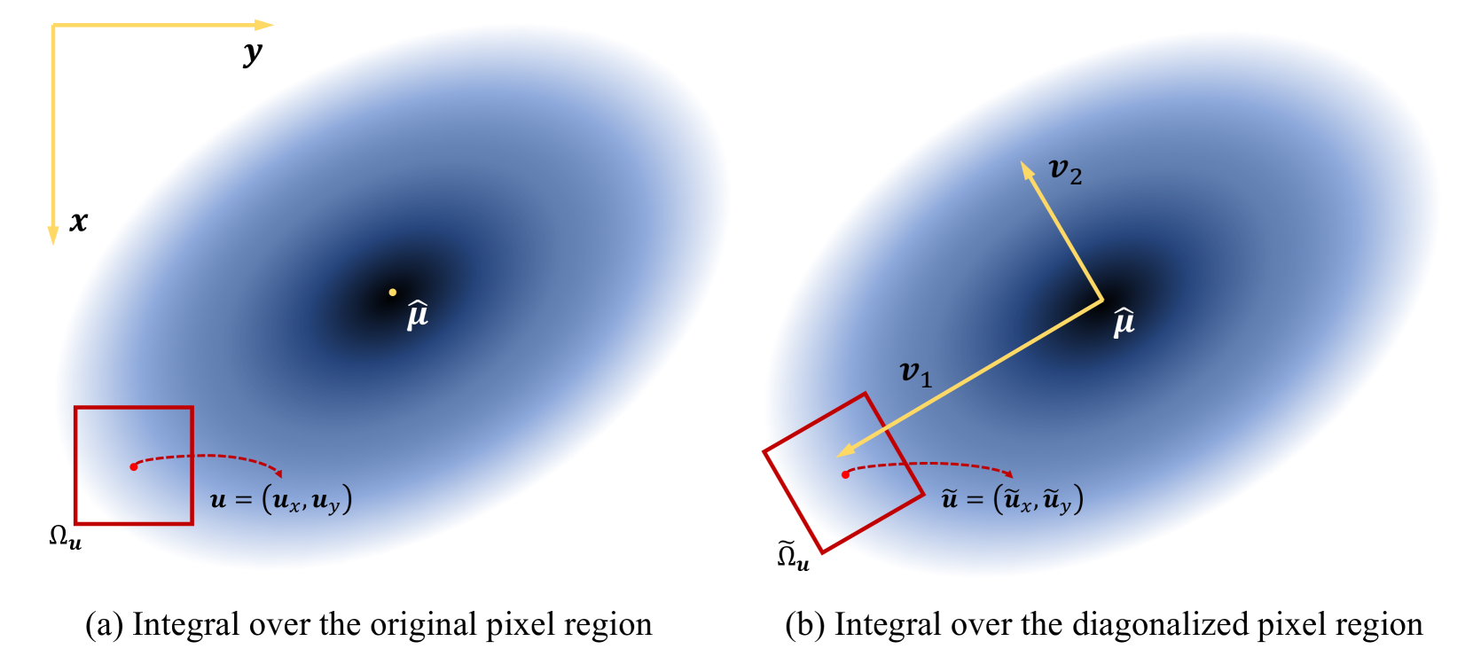
Figure 3:Example diagram of the pixel integration domain in Eq. 12 and the domain after rotation in Eq. 14. The yellow lines in Fig. 2(a) are the coordinate axes of 2D screen space; And the yellow lines in Fig. 2(b) are the eigenvectors scaled by the eigenvalues.
图3:等式3中的像素积分域的示例图。12和方程中旋转后的域。14.图2(a)中的黄线是2D屏幕空间的坐标轴;图2(B)中的黄线是由特征值缩放的特征向量。
4.2Analytic-Splatting
After revisiting the one-dimensional Gaussian signal integration, we tend to approximate the integral of projected 2D Gaussians within each pixel window area in Analytic-Splatting. Mathematically, we replace the sampled �2D(𝒖) in Eq. 4 with the approximated integral ℐ�2D(𝒖). For the pixel 𝒖=[��,��]⊤ in 2D screen space, which corresponds to the window area Ω𝒖 as shown in Fig. 2(a), the integration of Gaussian signal in Eq. 3 is represented as:
在重新访问一维高斯信号积分之后,我们倾向于近似解析溅射中每个像素窗口区域内投影的2D高斯的积分。在数学上,我们将采样的 �2D(𝒖) 替换为Eq. 4与近似积分 ℐ�2D(𝒖) 。对于2D屏幕空间中的像素 𝒖=[��,��]⊤ ,其对应于如图2(a)中所示的窗口区域 Ω𝒖 ,等式2(a)中的高斯信号的积分可以是:3表示为:
| ℐ�2D(𝒖)=∫��−12��+12∫��−12��+12exp(−�2(�−�^�)2−�2(�−�^�)2−�(�−�^�)(�−�^�)⏟correlation term)d�d�. | (12) |
Notably, handling the correlation term in this integral is intractable. To unravel the correlation term and thus feasibly solve the integral, we diagonalize the covariance matrix 𝚺^ of the 2D Gaussian �2D and slightly rotate the integration domain as shown in Fig. 2(b), thus approximating the integral by multiplying two independent 1D Gaussian integrals.
值得注意的是,处理该积分中的相关项是棘手的。为了解开相关项,从而可行地求解积分,我们对角化2D高斯 �2D 的协方差矩阵 𝚺^ ,并稍微旋转积分域,如图2(b)所示,从而通过乘以两个独立的1D高斯积分来近似积分。
In detail, we first perform eigenvalue decomposition on the covariance matrix 𝚺^ (refer to Eq. 5) to obtain eigenvalues {�1,�2} and the corresponding eigenvectors {𝒗1,𝒗2}. After diagonalization, for better description, we take 𝝁^=[�^�,�^�]⊤ (the mean vector of �2D) as the origin and the eigenvectors {𝒗1,𝒗2} as the axis to construct a new coordinate system.
详细地,我们首先对协方差矩阵 𝚺^ 执行特征值分解(参考等式100)。5)以获得特征值 {�1,�2} 和对应的特征向量 {𝒗1,𝒗2} 。对角化后,为了更好地描述,我们以 𝝁^=[�^�,�^�]⊤ ( �2D 的平均向量)为原点,以特征向量 {𝒗1,𝒗2} 为轴,构建一个新的坐标系。
In this coordinate system, given a pixel 𝒖=[��,��]⊤, we rewrite the �2D in Eq. 6 as the multiplication of two independent 1D Gaussians:
在该坐标系中,给定像素 𝒖=[��,��]⊤ ,我们将 �2D 重写为等式(1)。6作为两个独立的1D高斯的乘法:
| �2D(𝒖) | =exp(−12�1�~�2−12�2�~�2)=exp(−12�1�~�2)exp(−12�2�~�2), | (13) | ||
| 𝒖~ | =[�~��~�]=[−𝒗1−−𝒗2−](𝒖−𝝁^)=[−𝒗1−−𝒗2−][��−�^���−�^�], |
where 𝒖~=[�~�,�~�]⊤ denotes the diagonalized coordinate of the pixel center. After diagonalization, we further rotate the pixel integration domain Ω𝒖 along the pixel center to align it with the eigenvectors and get Ω~𝒖 for approximating the integral. Thus the integral in Eq. 12 can be approximated as:
其中 𝒖~=[�~�,�~�]⊤ 表示像素中心的对角化坐标。在对角化之后,我们进一步沿着像素中心沿着旋转像素积分域 Ω𝒖 以将其与特征向量对准,并且得到用于近似积分的 Ω~𝒖 。因此,在Eq. 12可以近似为:
| ℐ�2D(𝒖) | ≈∫Ω~𝒖�2D(𝒖)d𝒖=∫�~�−12�~�+12exp(−12�1�2)d�∫�~�−12�~�+12exp(−12�2�2)d� | (14) | ||
| =2��1�2∫�~�−12�~�+1212��1exp(−12�1�2)d�∫�~�−12�~�+1212��2exp(−12�2�2)d� | ||||
| ≈2��1�2[��1(�~�+12)−��1(�~�−12)][��2(�~�+12)−��2(�~�−12)]. |
where �∗ subscripts of � and � respectively correspond to Gaussian signals with the standard deviation �∗. �1=�1 and �2=�2 denote the standard derivations of the independent Gaussian signals along two eigenvectors respectively. In summary, the volume shading in Analytic-Splatting is given by:
其中 � 和 � 的下标 �∗ 分别对应于具有标准偏差 �∗ 的高斯信号。 �1=�1 和 �2=�2 分别表示独立高斯信号沿沿着两个特征向量的标准导数。总之,分析—溅射中的体积着色由下式给出:
| 𝑪(𝒖) | =∑�∈���ℐ�−�2D(𝒖|𝝁�^,𝚺�^)��𝒄�,��=∏�=1�−1(1−ℐ�−�2D(𝒖|𝝁�^,𝚺�^)��), | (15) | ||
| ℐ�2D(𝒖) | =2��1�2[��1(�~�+12)−��1(�~�−12)][��2(�~�+12)−��2(�~�−12)]. |
5Experiments 5实验
5.1Approximation Error Analysis
5.1近似误差分析
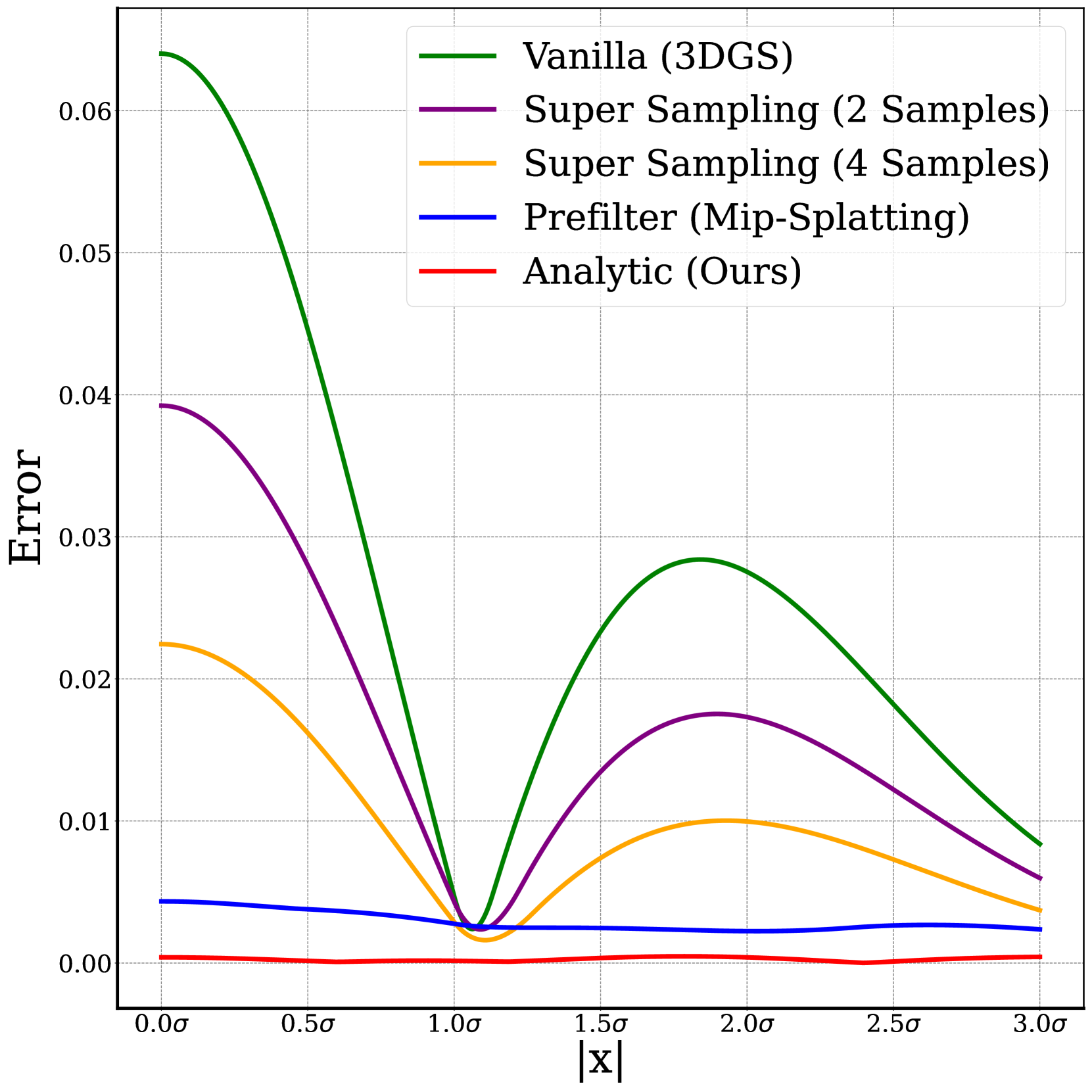
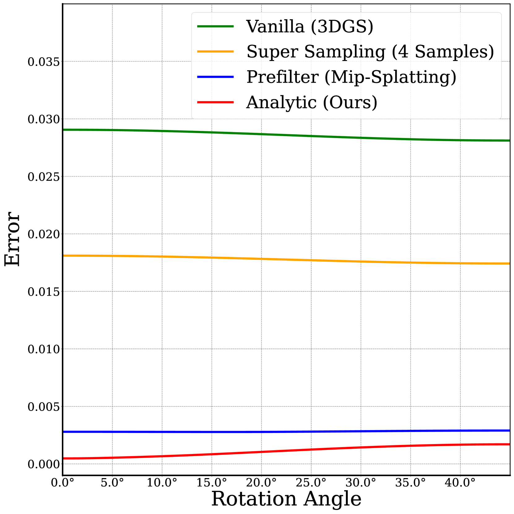
In this section, we first comprehensively explore the approximation errors in our scheme and then conduct an elaborate comparison against other schemes. It is worth noting that during training, the pruning and densification schemes proposed in 3DGS tend to maintain the standard deviations of Gaussian signals within an appropriate range (i.e. �∈[0.3,6.6]), and each Gaussian signal only responds to pixels within the 99% confidence interval (i.e. |�|<3�) for shading. Therefore, we only consider the Gaussian signals with standard deviations in [0.3,6.6], and merely discuss the approximation error of pixels within the 99% confidence interval.
在本节中,我们首先全面探讨我们的计划中的近似误差,然后与其他计划进行详细的比较。值得注意的是,在训练期间,3DGS中提出的修剪和致密化方案倾向于将高斯信号的标准偏差保持在适当的范围内(即 �∈[0.3,6.6] ),并且每个高斯信号仅响应于用于着色的 99% 置信区间(即 |�|<3� )内的像素。因此,我们只考虑在 [0.3,6.6] 中具有标准差的高斯信号,并且仅讨论在 99% 置信区间内的像素的近似误差。
Referring to Eq. 7 and Eq. 9, we get the approximation error function about the CDF of the Gaussian function:
参考方程式7、Eq。9,我们得到了关于高斯函数的CDF的逼近误差函数:
| ℰCDF(�)=|�(�)−�(�)|, | (16) |
and referring to Eq. 10 and Eq. 11, the approximation error function regarding the 1-width window area integral response is:
并参考Eq. 10、Eq. 11时,关于1宽度窗口面积积分响应的近似误差函数为:
| ℰInt(�)=|(�(�+12)−�(�+12))−(�(�+12)−�(�+12))|, | (17) |
the approximation error ℰCDF and ℰInt referring to different standard deviations are shown in Fig. 3(a) and Fig. 3(b) respectively. 33Since Eq. 16 and Eq. 17 are even functions, we show the results for the positive semi-axis over 0≤�≤6 in Fig. 4.
由于Eq. 16、Eq. 17是偶函数,我们在图4中示出了在 0≤�≤6 上的正半轴的结果。
图3(a)和图3(B)分别示出了涉及不同标准偏差的近似误差 ℰCDF 和 ℰInt 。 3 Please note that the errors shown in Fig. 4 are scaled by a tiny factor of 1e−4.
请注意,图4中所示的误差按微小的因子 1e−4 缩放。
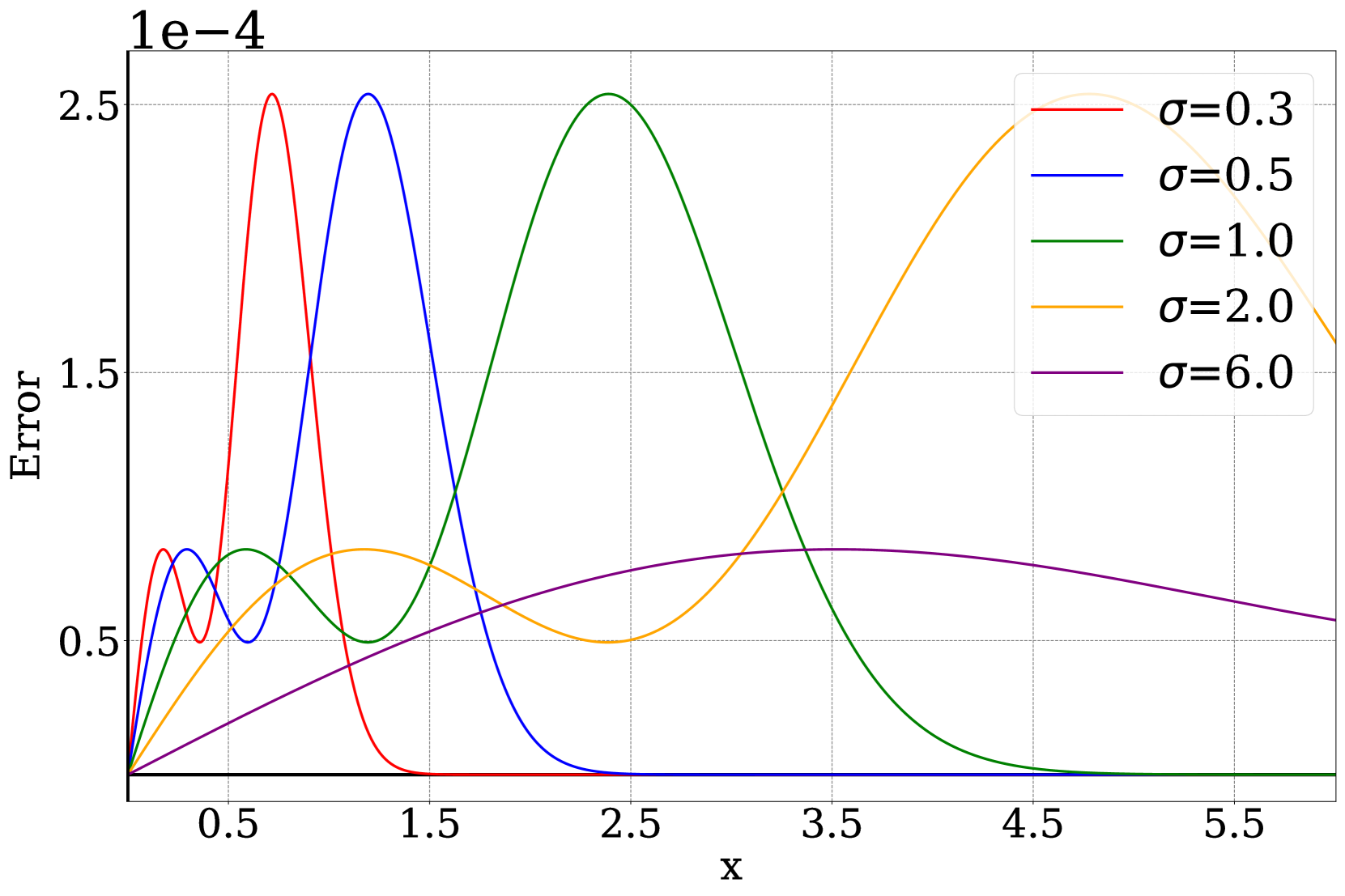
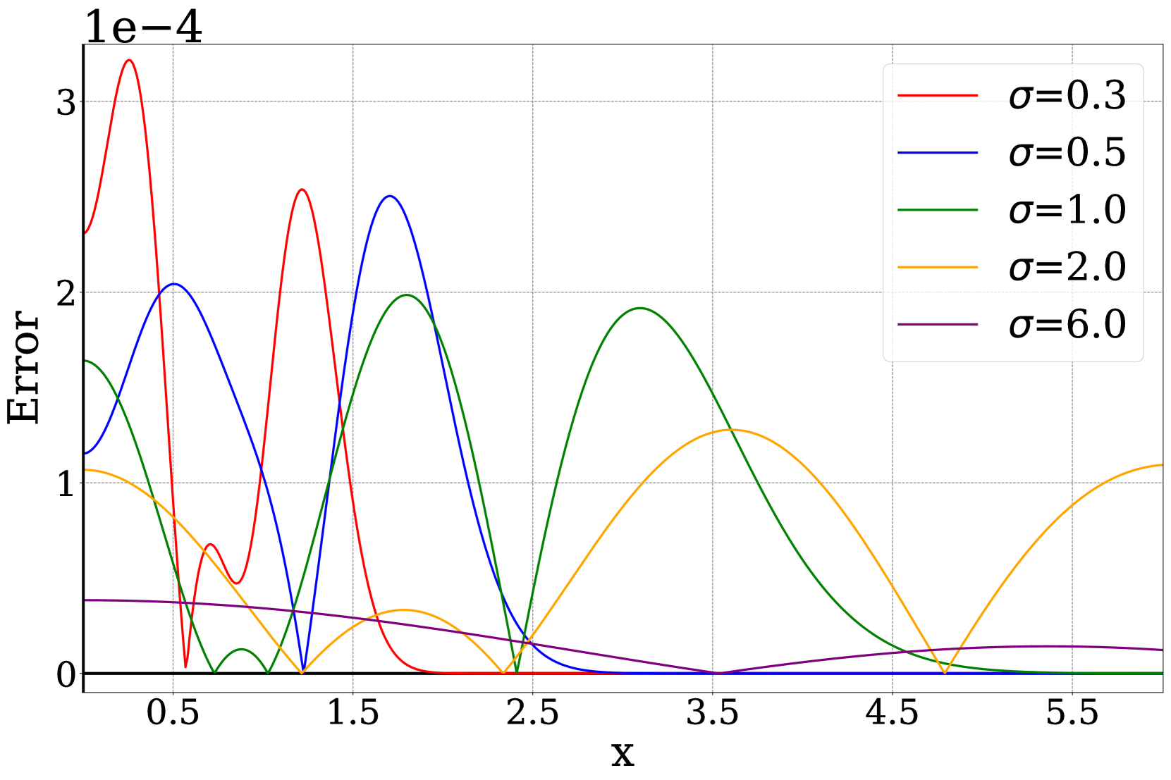
Figure 4:Error Analysis of using our conditioned logistic function Eq. 9 to approximate CDF of Gaussian signals Eq. 7 and window integration Eq. 10. Note that the scaling factor of the error is 1�−4.
图4:使用我们的条件逻辑函数Eq. 9来近似高斯信号的CDF 7和窗口积分方程。10.请注意,误差的比例因子为 1�−4 。
(a)Approximation errors referring to different standard variations.
(a)不同标准差的近似误差。
(b)Approximation errors for different variable distribution.
(b)不同变量分布的近似误差。
(c)Approximation errors of rotating the integral domain by different angles in Fig. 3.
(c)将积分域旋转不同角度的近似误差见图3。
Figure 5:Error Analysis of approximating the window integral Eq. 10 using different schemes in Fig. 2.
图5:近似窗口积分方程的误差分析图10使用图2中的不同方案。
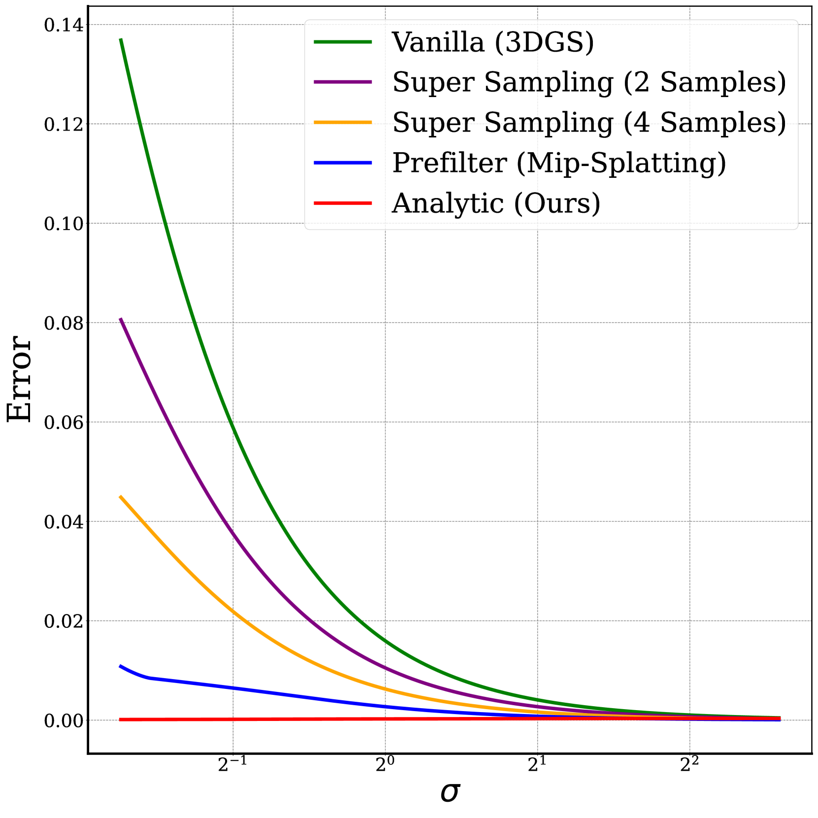
For approximating the integral response over the 1-width window area, our scheme significantly outperforms other schemes. Fig. 4(a) and Fig. 4(b) respectively show that one-dimensional approximation error with different standard deviations and variable distributions. Our scheme is robust to these two conditions, especially when the standard deviations of Gaussian signals become smaller, our advantage becomes more obvious, which means that our scheme is better at capturing the high-frequency signals (i.e. details) of the scene, and our subsequent experimental results also verify this.
对于近似的1宽度的窗口区域的积分响应,我们的计划显着优于其他计划。图4(a)和图4(B)分别示出了具有不同标准差和变量分布的一维近似误差。我们的方案对这两种情况都具有鲁棒性,尤其是当高斯信号的标准差变小时,我们的优势更加明显,这意味着我们的方案更好地捕捉场景的高频信号(即细节),我们后续的实验结果也验证了这一点。
| PSNR ↑ PSNR ↑ 的问题 | SSIM ↑ 阿信 ↑ | LPIPS ↓ LPIPPS ↓ 的问题 | |||||||||||||
| Full Res. | 1/2 Res. ◎片名Res. | 1/4 Res. ◎片名Res. | 1/8 Res. ◎片名Res. | Avg. | Full Res. | 1/2 Res. ◎片名Res. | 1/4 Res. ◎片名Res. | 1/8 Res. ◎片名Res. | Avg. | Full Res. | 1/2 Res. ◎片名Res. | 1/4 Res. ◎片名Res. | 1/8 Res. ◎片名Res. | Avg. | |
| NeRF w/o ℒarea 支持w/o # | 31.20 | 30.65 | 26.25 | 22.53 | 27.66 | 0.950 | 0.956 | 0.930 | 0.871 | 0.927 | 0.055 | 0.034 | 0.043 | 0.075 | 0.052 |
| NeRF [23] | 29.90 | 32.13 | 33.40 | 29.47 | 31.23 | 0.938 | 0.959 | 0.973 | 0.962 | 0.958 | 0.074 | 0.040 | 0.024 | 0.039 | 0.044 |
| MipNeRF [2] | 32.63 | 34.34 | 35.47 | 35.60 | 34.51 | 0.958 | 0.970 | 0.979 | 0.983 | 0.973 | 0.047 | 0.026 | 0.017 | 0.012 | 0.026 |
| Plenoxels [8] (Plenxels)[8] | 31.60 | 32.85 | 30.26 | 26.63 | 30.34 | 0.956 | 0.967 | 0.961 | 0.936 | 0.955 | 0.052 | 0.032 | 0.045 | 0.077 | 0.051 |
| TensoRF [5] | 32.11 | 33.03 | 30.45 | 26.80 | 30.60 | 0.956 | 0.966 | 0.962 | 0.939 | 0.956 | 0.056 | 0.038 | 0.047 | 0.076 | 0.054 |
| Instant-NGP [24] 快照NGP [ 24] | 30.00 | 32.15 | 33.31 | 29.35 | 31.20 | 0.939 | 0.961 | 0.974 | 0.963 | 0.959 | 0.079 | 0.043 | 0.026 | 0.040 | 0.047 |
| Tri-MipRF [13] MIRF [ 13] | 32.65 | 34.24 | 35.02 | 35.53 | 34.36 | 0.958 | 0.971 | 0.980 | 0.987 | 0.974 | 0.047 | 0.027 | 0.018 | 0.012 | 0.026 |
| 3DGS [16] | 28.79 | 30.66 | 31.64 | 27.98 | 29.77 | 0.943 | 0.962 | 0.972 | 0.960 | 0.960 | 0.065 | 0.038 | 0.025 | 0.031 | 0.040 |
| 3DGS-SS [16] | 32.05 | 33.78 | 33.92 | 31.12 | 32.71 | 0.964 | 0.975 | 0.980 | 0.977 | 0.974 | 0.039 | 0.021 | 0.016 | 0.020 | 0.024 |
| Mip-Splatting [36] [ 36]第三十六话 | 32.81 | 34.49 | 35.45 | 35.50 | 34.56 | 0.967 | 0.977 | 0.983 | 0.988 | 0.979 | 0.035 | 0.019 | 0.013 | 0.010 | 0.019 |
| Ours | 33.22 | 34.92 | 35.98 | 36.00 | 35.03 | 0.967 | 0.977 | 0.984 | 0.989 | 0.979 | 0.033 | 0.019 | 0.012 | 0.010 | 0.018 |
Table 1:Quantatitive Comparison of Analytic-Splatting against several cutting-edge methods on the multi-scale Blender Synthetic dataset [2]. These methods conduct multi-scale training and testing.
表1:分析溅射与多尺度Blender合成数据集上几种尖端方法的定量比较[ 2]。这些方法进行多尺度训练和测试。
Last but not least, we employ this scheme to approximate the window integral responses of two-dimensional Gaussian signals, which requires rotating the integration domain from Ω𝒖 to Ω~𝒖 as shown in Fig. 3 and inevitably introduces additional errors. To study this error, we record the approximation errors caused by rotating the integration domain from 0∘ to 45∘ 44Since we always hold �1≥�2 in practice, thus we only consider the approximation error caused by the rotation angle from 0∘ to 45∘.
由于我们在实践中总是保持 �1≥�2 ,因此我们只考虑由从 0∘ 到 45∘ 的旋转角度引起的近似误差。
最后但并非最不重要的是,我们采用该方案来近似二维高斯信号的窗口积分响应,这需要将积分域从 Ω𝒖 旋转到 Ω~𝒖 ,如图3所示,并且不可避免地引入额外的误差。为了研究这种误差,我们记录了将积分域从 0∘ 旋转到 45∘ 所引起的近似误差。 under different standard deviations of Gaussian signals and distributions, as shown in Fig. 4(c). Although the approximation error of our scheme slightly increases as the rotation angle becomes larger, our scheme still surpasses other schemes.
在高斯信号和分布的不同标准偏差下,如图4(c)所示。虽然我们的格式的近似误差随着旋转角的增大而略有增加,但我们的格式仍然优于其他格式。
5.2Comparison
To verify the anti-aliasing capability and versatility of Analytic-Splatting, we conduct experiments against state-of-the-art methods under the multi-scale training & multi-scale testing (MTMT) setting on Blender Synthetic [23, 2] and Mip-NeRF 360 [3] datasets. We further evaluate the performance of 3DGS and its variants under the super-resolution setting.
为了验证分析飞溅的抗锯齿能力和通用性,我们在Blender Synthetic [23,2]和Mip—NeRF 360 [3]数据集上的多尺度训练和多尺度测试(MTMT)设置下对最先进的方法进行了实验。我们进一步评估了3DGS及其变体在超分辨率设置下的性能。
Dataset & Metric. We conduct experiments using benchmark datasets of multi-scale Blender Synthetic [23, 2] and multi-scale Mip-NeRF 360 [3]. They respectively contain 8 objects and 9 scenes, each object and scene is compiled by downscaling the original dataset with a factor of 2, 4, and 8, and combining. For the Blender Synthetic dataset, each object contains 100 images for training and 200 images for testing. For the Mip-NeRF 360 dataset, we select 1 image from every 8 images for testing and the remaining images for training. To verify the efficacy of our method, we evaluate the synthesized novel view at multiple scales on both datasets in terms of Peak Signal-to-Noise Ratio (PSNR), Structural Similarity Index Measure (SSIM), and Learned Perceptual Image Path Similarity (LPIPS) [37].
数据集和指标。我们使用多尺度Blender Synthetic [ 23,2]和多尺度Mip-NeRF 360 [ 3]的基准数据集进行实验。它们分别包含8个对象和9个场景,每个对象和场景都是通过将原始数据集以2,4和8的因子进行缩减并组合来编译的。对于Blender Synthetic数据集,每个对象包含100张用于训练的图像和200张用于测试的图像。对于Mip-NeRF 360数据集,我们从每8张图像中选择1张图像进行测试,其余图像用于训练。为了验证我们的方法的有效性,我们根据峰值信噪比(PSNR)、结构相似性指数度量(SSIM)和学习感知图像路径相似性(LPIPS)在两个数据集上以多个尺度评估合成的新视图[ 37]。

Figure 6: Qualitative comparison of full-resolution and low-resolution (1/8) on Multi-Scale Blender [2]. All methods are trained on images with downsampling rates covering [1, 2, 4, 8]. Our method can better overcome the artifacts in 3DGS with better fidelity of details.
图6:多尺度混合器上全分辨率和低分辨率( 1/8 )的定性比较[ 2]。所有方法都是在下采样率覆盖[1,2,4,8]的图像上训练的。我们的方法可以更好地克服3DGS中的伪影,具有更好的细节保真度。
Implementation. We implement Analytic-Splatting upon 3DGS [16] and custom our shading module with CUDA extensions. Following 3DGS, we train Analytic-Splatting using the same parameters, training schedule, and loss functions, ensuring the efficacy of our scheme. To achieve super sampling of Gaussian signals, we implement 3DGS-SS, which first renders an image at twice the target resolution and obtains the final image at the target resolution through average pooling. For the MTMT setting, we follow previous works [2, 13, 36] and tend to select more full-resolution images as supervision samples during training. Please refer to supplementary material for more details on the backpropagation implementation of rendering.
实施.我们在3DGS [ 16]上实现了分析飞溅,并使用CUDA扩展自定义了我们的着色模块。在3DGS之后,我们使用相同的参数,训练时间表和损失函数训练分析-飞溅,以确保我们方案的有效性。为了实现高斯信号的超采样,我们实现了3DGS-SS,它首先以两倍的目标分辨率渲染图像,并通过平均池化获得目标分辨率的最终图像。对于MTMT设置,我们遵循以前的工作[ 2,13,36],并倾向于在训练期间选择更多的全分辨率图像作为监督样本。请参考补充资料,了解有关渲染的反向传播实现的更多详细信息。
| PSNR ↑ PSNR ↑ 的问题 | SSIM ↑ 阿信 ↑ | LPIPS ↓ LPIPPS ↓ 的问题 | |||||||||||||
| Full Res. | 1/2 Res. ◎片名Res. | 1/4 Res. ◎片名Res. | 1/8 Res. ◎片名Res. | Avg. | Full Res. | 1/2 Res. ◎片名Res. | 1/4 Res. ◎片名Res. | 1/8 Res. ◎片名Res. | Avg. | Full Res. | 1/2 Res. ◎片名Res. | 1/4 Res. ◎片名Res. | 1/8 Res. ◎片名Res. | Avg. | |
| Mip-NeRF 360 [3] | 27.50 | 29.19 | 30.45 | 30.86 | 29.50 | 0.778 | 0.864 | 0.912 | 0.931 | 0.871 | 0.254 | 0.136 | 0.077 | 0.058 | 0.131 |
| Mip-NeRF 360 + iNGP Mip—NeRF 360 + iNGP |
26.46 | 27.92 | 27.67 | 25.58 | 26.91 | 0.773 | 0.855 | 0.866 | 0.804 | 0.824 | 0.253 | 0.142 | 0.117 | 0.159 | 0.167 |
| Zip-NeRF [4] | 28.25 | 30.01 | 31.56 | 32.52 | 30.58 | 0.822 | 0.891 | 0.933 | 0.955 | 0.900 | 0.198 | 0.099 | 0.056 | 0.038 | 0.098 |
| 3DGS [16] | 26.55 | 28.00 | 28.51 | 27.45 | 27.63 | 0.779 | 0.854 | 0.891 | 0.888 | 0.853 | 0.274 | 0.162 | 0.102 | 0.087 | 0.156 |
| 3DGS-SS [16] | 27.20 | 28.75 | 29.89 | 29.71 | 28.89 | 0.800 | 0.871 | 0.914 | 0.928 | 0.878 | 0.246 | 0.138 | 0.081 | 0.061 | 0.131 |
| Mip-Splatting [36] [ 36]第三十六话 | 27.20 | 28.74 | 29.90 | 30.66 | 29.12 | 0.802 | 0.870 | 0.915 | 0.944 | 0.883 | 0.244 | 0.146 | 0.090 | 0.056 | 0.134 |
| Ours | 27.50 | 28.99 | 30.35 | 31.21 | 29.51 | 0.808 | 0.874 | 0.919 | 0.945 | 0.887 | 0.231 | 0.132 | 0.077 | 0.051 | 0.123 |
Table 2:Quantatitive Comparison of Analytic-Splatting against several cutting-edge methods on the multi-scale Mip-NeRF 360 dataset [3, 4]. These methods conduct multi-scale training and testing.
表2:在多尺度Mip—NeRF 360数据集上分析溅射与几种尖端方法的定量比较[3,4]。这些方法进行多尺度训练和测试。
Evaluation on Blender Synthetic Dataset. We compare our Analytic-Splatting with several state-of-the-art methods i.e. NeRF [23], MipNeRF [2], Plenoxels [8], TensoRF [5], Instant-NGP [24], Tri-MipRF [13], 3DGS [16] and its variants (i.e. 3DGS-SS, Mip-Splatting [36]) on the Blender Synthetic dataset. The quantitative results in Tab. 1 show that Analytic-Splatting outperforms other methods in all aspects. The qualitative results in Fig. 6 demonstrate that Analytic-Splatting can better capture high-frequency details while being anti-aliased. More results can be found in the supplementary material.
Blender合成数据集的评估。我们将我们的分析飞溅与几种最先进的方法进行比较,即NeRF [ 23],MipNeRF [ 2],Plenoxels [ 8],TensoRF [ 5],Instant-NGP [ 24],Tri-MipRF [ 13],3DGS [ 16]及其变体(即3DGS-SS,Mip-Splatting [ 36])在Blender合成数据集上。表中的定量结果。1表明,分析飞溅优于其他方法在各个方面。图6中的定性结果表明,分析飞溅可以更好地捕捉高频细节,同时进行抗锯齿。更多的结果可以在补充材料中找到。

Figure 7:Qualitative comparisons of full-resolution and low-resolution on Multi-Scale Mip-NeRF 360. [3, 4] All methods are trained on images with downsampling rates covering [1, 2, 4, 8]. Our method can better overcome the artifacts with better fidelity of details. Please note that the artifacts of 3DGS/3DGS-SS become obvious at low resolutions, especially on elongated shapes (e.g. wheels and flower stems), while Mip-Splatting produces over-smoothing results (e.g. lobes).
图7:多尺度Mip-NeRF 360上全分辨率和低分辨率的定性比较。[ 3,4]所有方法都是在下采样率覆盖[1,2,4,8]的图像上训练的。我们的方法可以更好地克服伪影,具有更好的细节保真度。请注意,3DGS/3DGS-SS的伪影在低分辨率下变得明显,特别是在细长形状(例如车轮和花茎)上,而Mip-Splatting会产生过度平滑的结果(例如叶片)。
Evaluation on Mip-NeRF 360 Dataset. We compare our Analytic-Splatting with several cut-edge methods i.e. Mip-NeRF 360 and its iNGP encoding version [3], Zip-NeRF [4], 3DGS [16] and its variants (i.e. 3DGS-SS, Mip-Splatting [36]) on the challenging Mip-NeRF 360 dataset. The results of Zip-NeRF are reported from the available official implementation 55GitHub - jonbarron/camp_zipnerf
Mip—NeRF 360数据集的评估。我们将我们的分析飞溅与几种切割边缘方法进行比较,即Mip—NeRF 360及其iNGP编码版本[3],Zip—NeRF [4],3DGS [16]及其变体(即3DGS—SS,Mip—Splatting [36])在具有挑战性的Mip—NeRF 360数据集上。Zip—NeRF的结果来自可用的官方实现 5. Please note that Mip-NeRF 360 and Zip-NeRF struggle with real-time rendering, especially Zip-NeRF performs supersampling techniques in the rendering phase. The quantitative results in Tab. 2 show that our method is second only to Zip-NeRF, and we outperform other methods with real-time rendering capability (i.e. 3DGS and its variants). The qualitative comparisons in Fig. 7 demonstrate that our method has better anti-aliasing capability and detail fidelity despite facing complex scenes. More results can be found in the supplementary material.
.请注意,Mip—NeRF 360和Zip—NeRF在实时渲染方面存在困难,特别是Zip—NeRF在渲染阶段执行了超分辨率技术。表中的定量结果。2表明,我们的方法是仅次于Zip—NeRF,我们优于其他方法的实时渲染能力(即3DGS及其变体)。图7中的定性比较表明,我们的方法具有更好的抗锯齿能力和细节保真度,即使面对复杂的场景。更多的结果可以在补充材料中找到。
Super-Resolution Evaluation on Mip-NeRF 360 Dataset. We further evaluate our method against other 3DGS and its variants under the super-resolution setting (2× Res.) on the Mip-NeRF 360 dataset. All methods are trained on the Multi-Scale Mip-NeRF 360 dataset. The quantitative results are shown in Tab. 3 and the qualitative results are shown in Fig. 8. Both results demonstrate the superior performance of our method, further supporting the capability of Analytic-Splatting in capturing details. Conversely, Mip-Splatting is insufficient in capturing details due to pre-filtering.
Mip-NeRF 360数据集的超分辨率评估我们进一步评估我们的方法对其他3DGS及其变体下的超分辨率设置( 2× Res.)在Mip-NeRF 360数据集上。所有方法都是在Multi-Scale Mip-NeRF 360数据集上训练的。定量结果见表1。图3中示出了定性结果,图8中示出了定性结果。这两个结果都证明了我们的方法的上级性能,进一步支持了分析飞溅捕捉细节的能力。相反,由于预过滤,Mip-Splatting在捕获细节方面是不够的。
| PSNR ↑ PSNR ↑ 的问题 | ||||||||||
| bicycle | flowers | garden | stump | treehill | room | counter | kitchen | bonsai | Avg. | |
| 3DGS | 23.14 | 20.28 | 24.62 | 25.44 | 21.90 | 30.27 | 28.08 | 29.51 | 30.34 | 25.95 |
| 3DGS-SS | 23.98 | 20.84 | 25.48 | 26.24 | 22.12 | 30.90 | 28.69 | 30.53 | 31.34 | 26.68 |
| Mip-Splatting Mip—Splating | 23.82 | 20.60 | 24.97 | 25.78 | 21.82 | 30.95 | 28.68 | 30.45 | 31.07 | 26.46 |
| Ours | 24.22 | 20.97 | 25.72 | 26.29 | 22.04 | 31.04 | 28.90 | 31.10 | 31.83 | 26.90 |
| SSIM ↑ 阿信 ↑ | ||||||||||
| bicycle | flowers | garden | stump | treehill | room | counter | kitchen | bonsai | Avg. | |
| 3DGS | 0.639 | 0.492 | 0.707 | 0.706 | 0.578 | 0.902 | 0.891 | 0.893 | 0.916 | 0.747 |
| 3DGS-SS | 0.675 | 0.527 | 0.747 | 0.739 | 0.596 | 0.908 | 0.901 | 0.907 | 0.926 | 0.769 |
| Mip-Splatting Mip—Splating | 0.671 | 0.526 | 0.737 | 0.728 | 0.589 | 0.906 | 0.898 | 0.900 | 0.924 | 0.764 |
| Ours | 0.683 | 0.535 | 0.761 | 0.739 | 0.596 | 0.910 | 0.904 | 0.911 | 0.930 | 0.774 |
| LPIPS ↓ LPIPPS ↓ 的问题 | ||||||||||
| bicycle | flowers | garden | stump | treehill | room | counter | kitchen | bonsai | Avg. | |
| 3DGS | 0.382 | 0.471 | 0.325 | 0.378 | 0.462 | 0.324 | 0.314 | 0.241 | 0.321 | 0.358 |
| 3DGS-SS | 0.345 | 0.438 | 0.281 | 0.340 | 0.435 | 0.314 | 0.297 | 0.220 | 0.307 | 0.333 |
| Mip-Splatting Mip—Splating | 0.341 | 0.433 | 0.291 | 0.338 | 0.439 | 0.309 | 0.295 | 0.216 | 0.300 | 0.329 |
| Ours | 0.342 | 0.429 | 0.268 | 0.338 | 0.434 | 0.307 | 0.291 | 0.209 | 0.300 | 0.324 |
Table 3:Quantatitive comparison of super-resolution (2×) on Multi-Scale Mip-NeRF 360. [3, 4] All methods are trained on images with downsampling rates covering [1, 2, 4, 8]. we boldly mark the best results.
表3:多尺度Mip—NeRF 360上的超分辨率(2 × )的定量比较。[3,4]所有方法都是在下采样率覆盖[1,2,4,8]的图像上训练的。我们大胆地标记最好的结果。

Figure 8:Qualitative comparison of super-resolution (2×) on Multi-Scale Mip-NeRF 360. [3, 4] All methods are trained on images with downsampling rates covering [1, 2, 4, 8]. Please note the high-frequency aliasing of 3DGS-SS and the over-smoothing of Mip-Splatting. Our results are closest to the ground truth.
图8:多尺度Mip-NeRF 360上的超分辨率(2 × )的定性比较。[ 3,4]所有方法都是在下采样率覆盖[1,2,4,8]的图像上训练的。请注意3DGS-SS的高频混叠和Mip-Splatting的过度平滑。我们的结果最接近真实情况。
6Conclusion 六、结论
In this paper, we first revisit the window response of one-dimensional Gaussian signals and reason about an analytical and accurate approximation using a conditioned logistic function. We then introduce this approximation in the two-dimensional pixel shading and present Analytic-Splatting, which approximates the pixel area integral response to achieve anti-aliasing capability and better detail fidelity. Our extensive experiments demonstrate the efficacy of Analytic-Splatting in achieving state-of-the-art novel view synthesis results under multi-scale and super-resolution settings.
在本文中,我们首先回顾了一维高斯信号的窗口响应和原因的分析和准确的近似使用条件逻辑函数。然后,我们在二维像素着色中引入这种近似,并提出了解析飞溅,它近似像素面积积分响应,以实现抗锯齿能力和更好的细节保真度。我们广泛的实验证明了分析溅射在多尺度和超分辨率设置下实现最先进的新颖视图合成结果的功效。