小土堆pytorch--损失函数与反向传播

一级目录

二级目录

三级目录

损失函数与反向传播

1. 损失函数用法说明

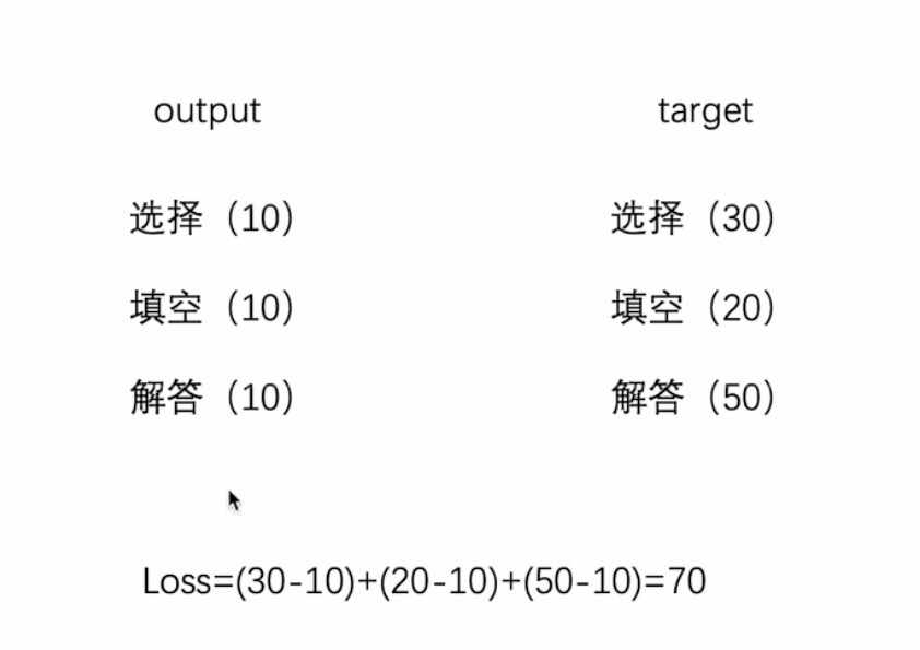
我们举个例子，假如一张考试卷满分100分，其中选择30分，填空20分，解答50分
但是某位同学考了30分，这三项都是10分，满分与考试成绩的差距就叫做损失

作用：

1. 计算实际输出和目标之间的差距
2. 为我们更新输出提供了一定的依据

1.1 L1LOSS

这是pytorch官网对于L1Loss的说明


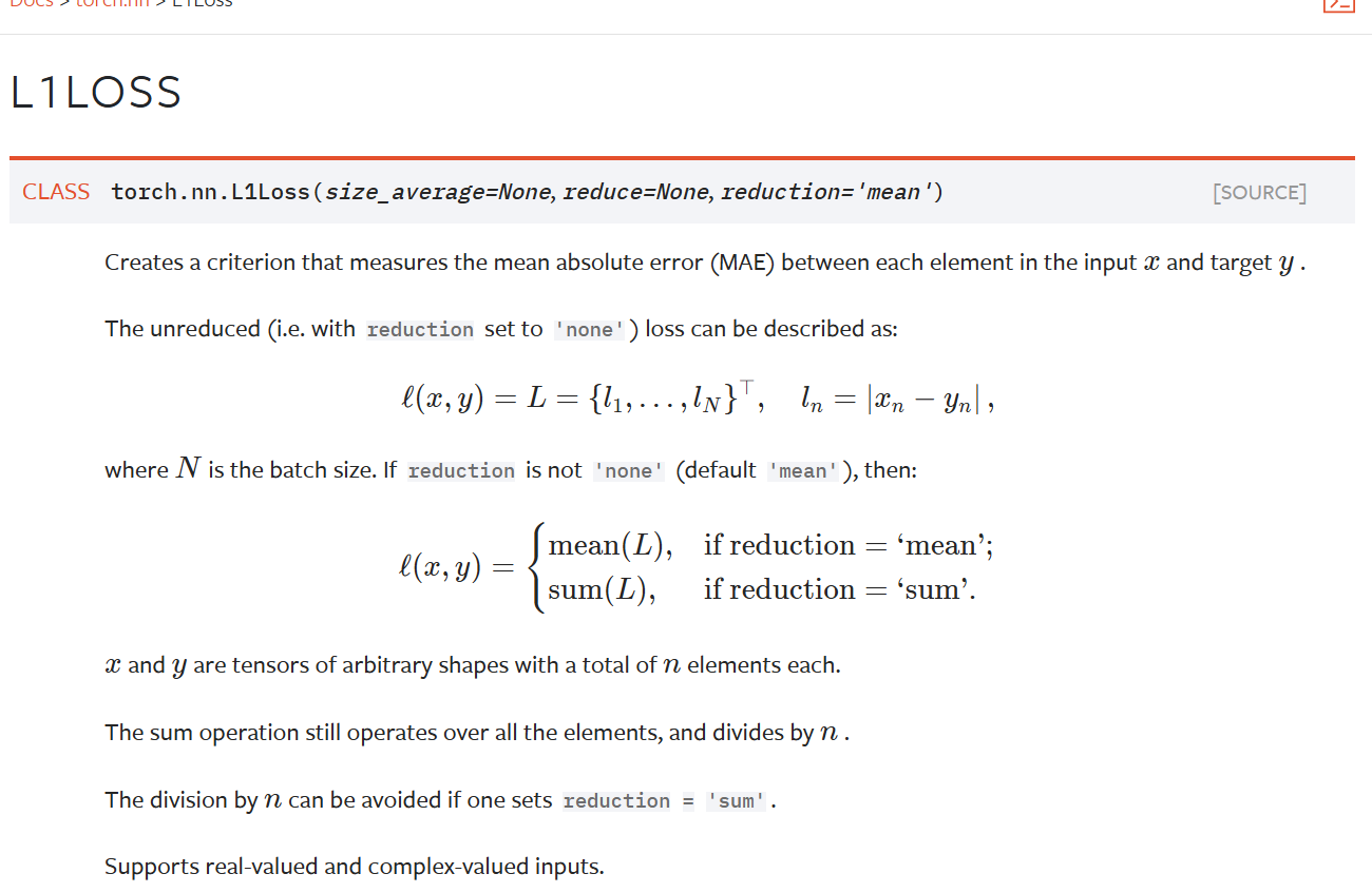
这是PyTorch中 nn.L1Loss 类的文档说明，用于计算平均绝对误差损失：

功能

度量输入张量 x 和目标张量 y 对应元素间的平均绝对误差（MAE ）。

公式及参数

• 未规约情况（reduction='none'） ：对每个样本计算损失，公式为 $l_n=|x_n-y_n|$ ，得到损失向量 L = { l 1 , . . . , l N } T L = \{l_1, ..., l_N\}^T L={l1​,...,lN​}T ，$N$ 是批量大小。
• 规约情况 ：
  • reduction='mean' （默认 ）：对损失向量求均值，计算所有元素损失平均值。
  • reduction='sum' ：对损失向量求和，得到所有元素损失总和。

输入要求

x 和 y 是形状任意但需相同、元素总数相同的张量，支持实值和复值输入。

已弃用参数

size_average 和 reduce 已弃用，指定它们会覆盖 reduction 参数设置，推荐使用 reduction 来确定损失规约方式。

形状要求

输入和目标张量形状为 (N, *) ，N 是批量大小， * 代表任意额外维度；若 reduction='none' ，输出形状与输入相同，否则输出为标量。

import torch
from torch.nn import L1Loss

inputs = torch.tensor([1,2,3], dtype = torch.float32)
targets = torch.tensor([1,2,5], dtype = torch.float32)

inputs = torch.reshape(inputs,(1,1,1,3))
targets = torch.reshape(targets, (1,1,1,3))

loss = L1Loss()
result = loss(inputs, targets)

print(result)

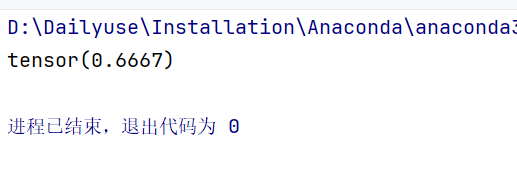
运行结果为

import torch
from torch.nn import L1Loss

inputs = torch.tensor([1,2,3], dtype = torch.float32)
targets = torch.tensor([1,2,5], dtype = torch.float32)

inputs = torch.reshape(inputs,(1,1,1,3))
targets = torch.reshape(targets, (1,1,1,3))

loss = L1Loss(reduction="sum")
result = loss(inputs, targets)

print(result)

换成sum的模式，就是求损失的和了

1.2 MSELOSS

这是关于PyTorch中 nn.MSELoss 类的说明，用于计算均方误差损失：

功能

衡量输入张量 x 和目标张量 y 对应元素间的均方误差（即L2范数的平方 ）。

公式及参数

• 未规约情况（reduction='none'） ：对每个样本计算损失，公式为 $l_n=(x_n-y_n{)}^2$ ，得到损失向量 L = { l 1 , . . . , l N } T L = \{l_1, ..., l_N\}^T L={l1​,...,lN​}T ，$N$ 是批量大小。
• 规约情况 ：
  • reduction='mean' （默认 ）：对损失向量求均值，即计算所有元素损失的平均值。
  • reduction='sum' ：对损失向量求和，得到所有元素损失总和。

输入要求

x 和 y 是形状任意的张量，且元素总数相同。

import torch
from torch.nn import L1Loss, MSELoss

inputs = torch.tensor([1,2,3], dtype = torch.float32)
targets = torch.tensor([1,2,5], dtype = torch.float32)

inputs = torch.reshape(inputs,(1,1,1,3))
targets = torch.reshape(targets, (1,1,1,3))

loss = L1Loss(reduction="sum")
result = loss(inputs, targets)

print(result)

loss = MSELoss(reduction="sum")
result = loss(inputs, targets)

print(result)

运行结果

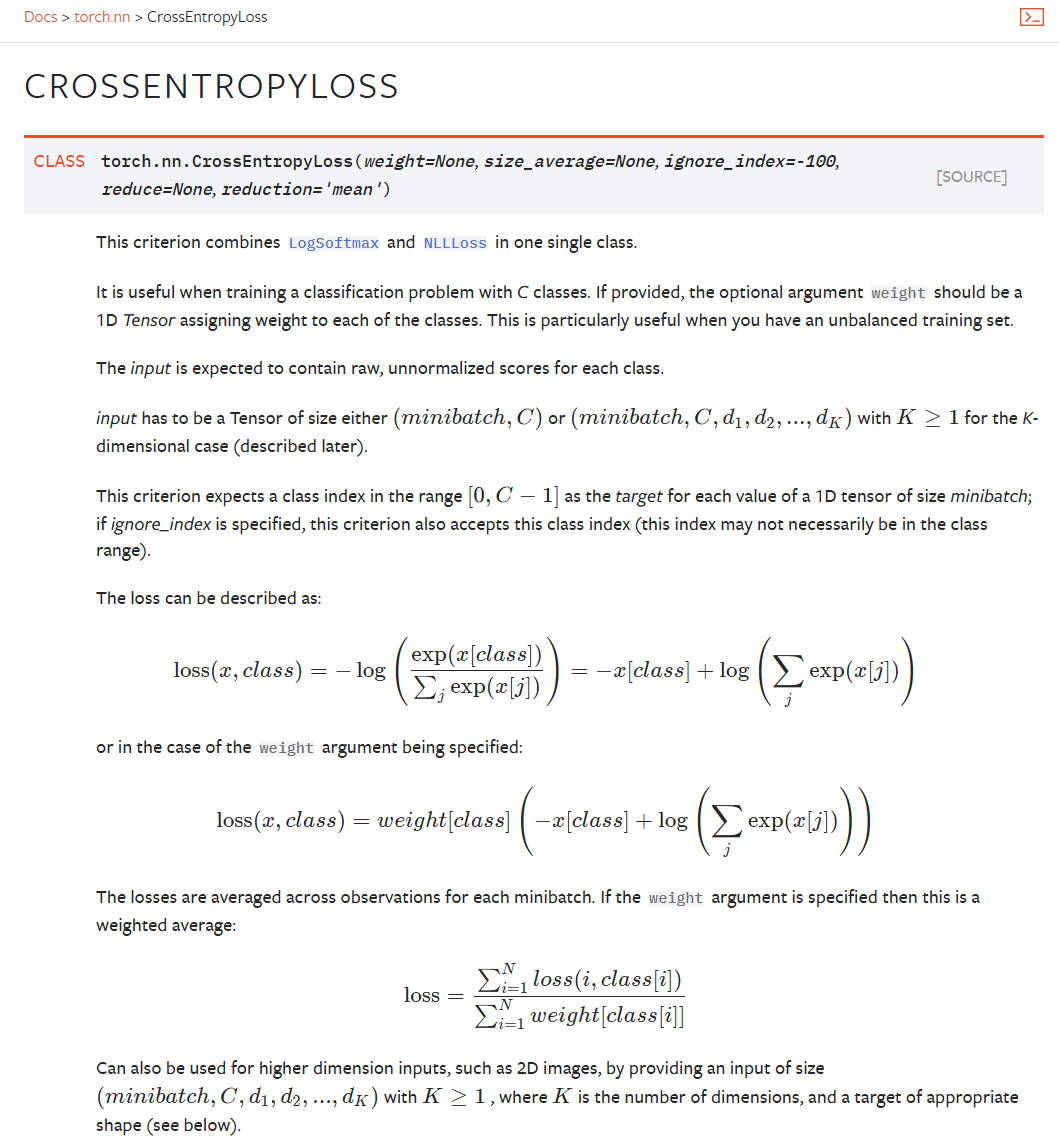
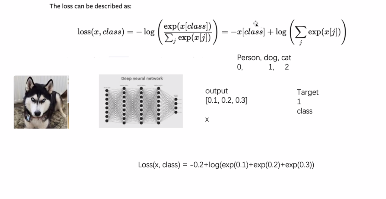
1.3 交叉熵损失函数

一般用于多分类问题

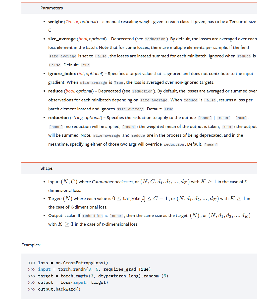
这是PyTorch中 nn.CrossEntropyLoss 类的相关说明，用于分类问题损失计算：

功能与原理

• 将 LogSoftmax 和 NLLLoss 融合在一个类中，适用于C个类别的分类训练任务。输入是每个类别的原始未归一化分数，目标是类别索引。
• 计算公式：未指定权重时，$loss(x,class)=-log(\frac{exp(x[class])}{{\sum }_{j}exp(x[j])})=-x[class]+log({\sum }_{j}exp(x[j]))$ ；指定权重 weight 时，$loss(x,class)=weight[class](-x[class]+log({\sum }_{j}exp(x[j])))$ ，最后对小批量样本损失进行平均或求和。

参数

• weight （可选）：手动为每个类指定重缩放权重，是大小为C（类别数）的1D张量，处理训练集类别不均衡时有用。
• size_average 、reduce ：已弃用，分别涉及损失平均或求和相关功能，指定它们会覆盖 reduction 。
• ignore_index （可选）：指定被忽略的目标值，其不参与输入梯度计算， size_average=True 时，损失在非忽略目标上平均。
• reduction （可选）：确定输出的规约方式，'none' 不规约，'mean' 求加权均值（默认 ），'sum' 求和。

形状要求

• 输入：形状为 (N, C) 或 (N, C, d1, d2, ..., dk) （$K\ge 1$ ，用于高维情况），N 是批量大小，C 是分类的类别数。
• 目标：形状为 (N) 或 (N, d1, d2, ..., dk) （$K\ge 1$ ），值在 0 到 C - 1 范围。
• 输出：reduction='none' 时与目标形状相同，否则为标量。

import torch
from torch import nn
from torch.nn import L1Loss, MSELoss

# inputs = torch.tensor([1,2,3], dtype = torch.float32)
# targets = torch.tensor([1,2,5], dtype = torch.float32)
#
# inputs = torch.reshape(inputs,(1,1,1,3))
# targets = torch.reshape(targets, (1,1,1,3))
#
# loss = L1Loss(reduction="sum")
# result = loss(inputs, targets)
#
# print(result)
#
# loss = MSELoss(reduction="sum")
# result = loss(inputs, targets)
#
# print(result)

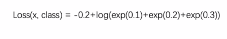
x = torch.tensor([0.1,0.2,0.3])
y = torch.tensor([1])
x = torch.reshape(x, (1,3))
loss_cross = nn.CrossEntropyLoss()
result = loss_cross(x, y)
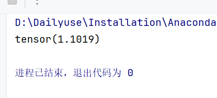
print(result)

总结一下：

1. loss function 要根据需求（要解决的问题）来使用
2. 要注意输入输出

2. 反向传播

概念

反向传播（Backpropagation）是一种在神经网络训练中计算梯度的方法 。神经网络训练的目标是调整参数（权重和偏置 ），使网络输出尽可能接近真实标签，而反向传播能高效计算参数的梯度，基于梯度来调整参数。

工作原理

1. 前向传播：输入数据进入神经网络，依次经过各个隐藏层，最后到达输出层得到输出结果。比如图像识别任务中，图像数据输入，经多层处理得到各类别的预测概率。
2. 计算损失：用损失函数（如前面介绍的交叉熵损失等 ）衡量预测结果和真实标签的差距。损失反映了当前网络预测的好坏程度。
3. 反向传播：从输出层开始，将损失关于输出的梯度反向传播回网络的输入层。依据链式法则，计算损失对每一层参数（权重和偏置 ）的梯度。例如在一个简单的两层神经网络中，先算出损失对第二层参数的梯度，再通过链式法则算出对第一层参数的梯度 。
4. 参数更新：根据计算出的梯度，使用优化算法（如随机梯度下降 ）来更新神经网络的参数。梯度指示了参数调整的方向和幅度，通常沿着梯度反方向调整参数，使损失降低。

直观理解

可以把神经网络想象成一个复杂的函数，输入数据经函数运算得到输出。反向传播就像是告诉这个函数，它哪里算得不对，通过计算梯度指出参数如何调整能让计算结果更准确，然后不断调整参数，让函数计算得越来越好。

import torchvision
from torch import nn
from torch.nn import Sequential, Conv2d, MaxPool2d, Flatten, Linear
from torch.utils.data import DataLoader

dataset = torchvision.datasets.CIFAR10("das",train=False,transform=torchvision.transforms.ToTensor(),
                                       download=True)
dataloader = DataLoader(dataset, batch_size=64)

class Test(nn.Module):
    def __init__(self):
        super(Test,self).__init__()
        self.model1 = Sequential(
            Conv2d(3,32,5,padding=2),
            MaxPool2d(2),
            Conv2d(32, 32, 5, padding=2),
            MaxPool2d(2),
            Conv2d(32, 64, 5, padding=2),
            MaxPool2d(2),
            Flatten(),
            Linear(1024, 64),
            Linear(64, 10)
        )

    def forward(self,x):
        x = self.model1(x)
        return x

loss = nn.CrossEntropyLoss()
test = Test()
for data in dataloader:
    imgs, targets = data
    outputs = test(imgs)
    result_loss = loss(outputs,targets)
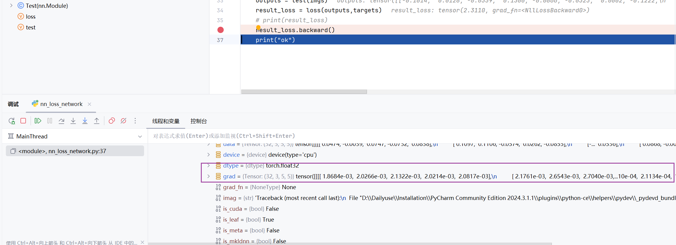
    # print(result_loss)
    result_loss.backward()
    print("ok")

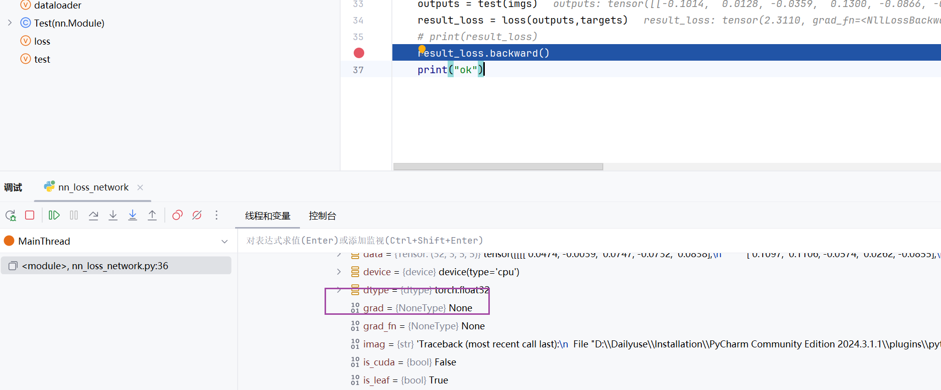
可以看到往下走了一行是，自动更新出梯度的参数

下一节我们会使用优化算法（如随机梯度下降 ）来更新神经网络的参数