- 预训练的概念
- 常见的分类预训练模型
- 图像预训练模型的发展史
- 预训练的策略
- 预训练代码实战:resnet18
作业:
- 尝试在cifar10对比如下其他的预训练模型,观察差异,尽可能和他人选择的不同
- 尝试通过ctrl进入resnet的内部,观察残差究竟是什么
一、预训练的概念
因为准确率最开始随着epoch的增加而增加,随着循环的更新,参数在不断发生更新
所以参数的初始值对训练结果有很大的影响:如果最开始的初始值比较好,后续训练的轮数就会少很多,不同的初始值可能会导致陷入不同的局部最优解
所以如果最开始能有比较好的参数,即可能导致未来训练次数少,也可能导致未来训练避免陷入局部最优解的问题。由此引出预训练模型。
1. 那为什么要选择类似任务的数据集预训练的模型参数呢?
因为任务差不多,他提取特征的能力才有用,如果任务相差太大,他的特征提取能力就没那么好。
所以本质预训练就是拿别人已经具备的通用特征提取能力来接着强化能力使之更加适应我们的数据集和任务。
2. 为什么要求预训练模型是在大规模数据集上训练的,小规模不行么?
因为提取的是通用特征,所以如果数据集数据少、尺寸小,就很难支撑复杂任务学习通用的数据特征。比如你是一个物理的博士,让你去做小学数学题,很快就能上手;但是你是一个小学数学速算高手,让你做物理博士的课题,就很困难。所以预训练模型一般就挺强的。
我们把用预训练模型的参数,然后接着在自己数据集上训练来调整该参数的过程叫做微调,这种思想叫做迁移学习。把预训练的过程叫做上游任务,把微调的过程叫做下游任务。
这里给大家介绍一个常常用来做预训练的数据集,ImageNet,ImageNet 1000 个类别,有 1.2 亿张图像,尺寸 224x224,数据集大小 1.4G,下载地址:http://www.image-net.org/。
二、经典的预训练模型
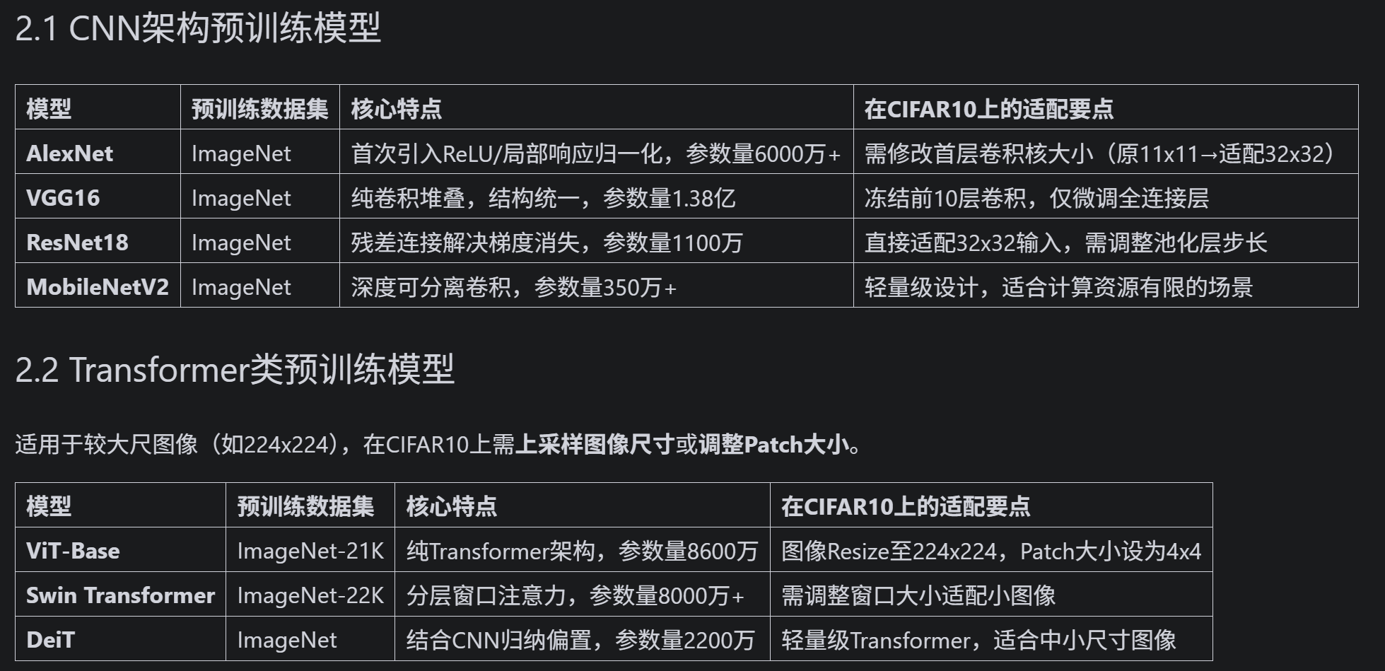

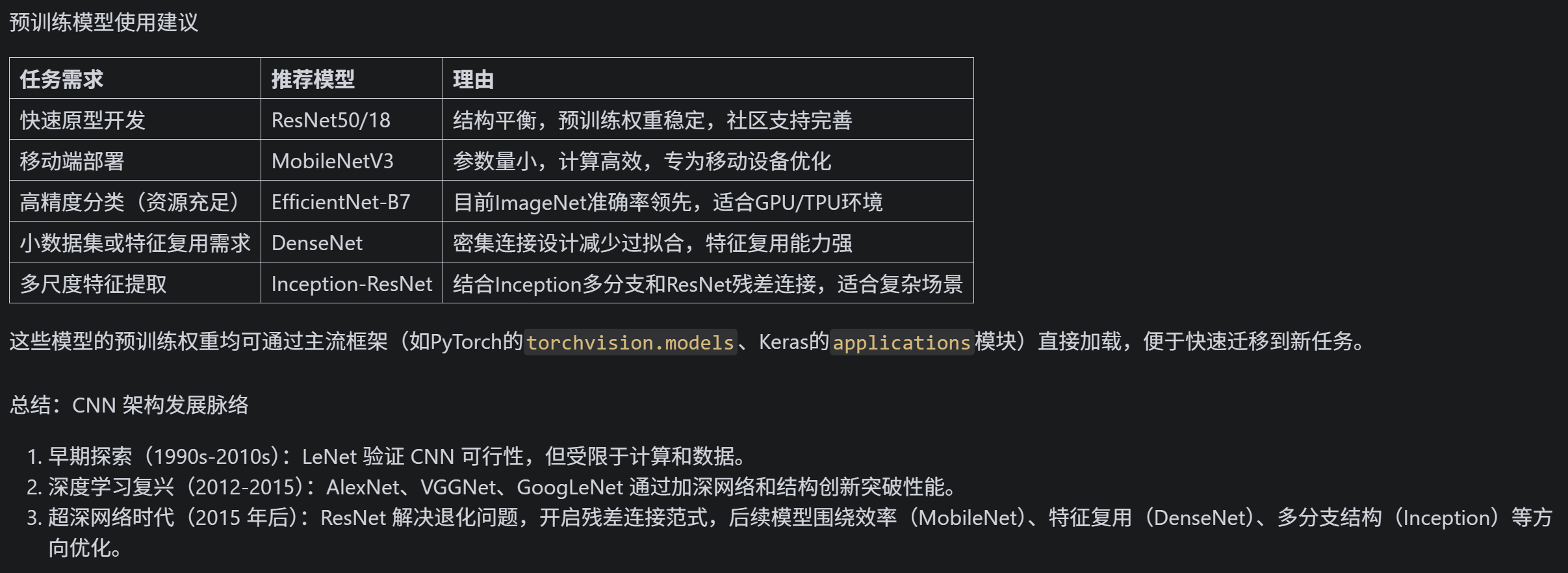
三、常见的分类预训练模型介绍
训练策略
那么什么模型会被选为预训练模型呢?比如一些调参后表现很好的cnn神经网络(固定的神经元个数+固定的层数等)。
所以调用预训练模型做微调,本质就是 用这些固定的结构+之前训练好的参数 接着训练
所以需要找到预训练的模型结构并且加载模型参数
相较于之前用自己定义的模型有以下几个注意点
1. 需要调用预训练模型和加载权重
2. 需要resize 图片让其可以适配模型
3. 需要修改最后的全连接层以适应数据集
其中,训练过程中,为了不破坏最开始的特征提取器的参数,最开始往往先冻结住特征提取器的参数,然后训练全连接层,大约在5-10个epoch后解冻训练。
主要做特征提取的部分叫做backbone骨干网络;负责融合提取的特征的部分叫做Featue Pyramid Network(FPN);负责输出的预测部分的叫做Head。
import torch
import torch.nn as nn
import torch.optim as optim
from torchvision import datasets, transforms, models
from torch.utils.data import DataLoader
import matplotlib.pyplot as plt
import os

# 设置中文字体支持
plt.rcParams["font.family"] = ["SimHei"]
plt.rcParams['axes.unicode_minus'] = False  # 解决负号显示问题

# 检查GPU是否可用
device = torch.device("cuda" if torch.cuda.is_available() else "cpu")
print(f"使用设备: {device}")

# 1. 数据预处理(训练集增强,测试集标准化)
train_transform = transforms.Compose([
    transforms.RandomCrop(32, padding=4),
    transforms.RandomHorizontalFlip(),
    transforms.ColorJitter(brightness=0.2, contrast=0.2, saturation=0.2, hue=0.1),
    transforms.RandomRotation(15),
    transforms.ToTensor(),
    transforms.Normalize((0.4914, 0.4822, 0.4465), (0.2023, 0.1994, 0.2010))
])

test_transform = transforms.Compose([
    transforms.ToTensor(),
    transforms.Normalize((0.4914, 0.4822, 0.4465), (0.2023, 0.1994, 0.2010))
])

# 2. 加载CIFAR-10数据集
train_dataset = datasets.CIFAR10(
    root='./data',
    train=True,
    download=True,
    transform=train_transform
)

test_dataset = datasets.CIFAR10(
    root='./data',
    train=False,
    transform=test_transform
)

# 3. 创建数据加载器
batch_size = 64
train_loader = DataLoader(train_dataset, batch_size=batch_size, shuffle=True)
test_loader = DataLoader(test_dataset, batch_size=batch_size, shuffle=False)

# 4. 定义MobileNetV2模型(替代ResNet18)
def create_mobilenetv2(pretrained=True, num_classes=10):
    # 创建MobileNetV2模型
    model = models.mobilenet_v2(pretrained=pretrained)

    # 修改最后一层分类器
    # MobileNetV2的分类器结构与ResNet不同,需要特别注意
    in_features = model.classifier[1].in_features
    model.classifier[1] = nn.Linear(in_features, num_classes)

    return model.to(device)

# 5. 冻结/解冻模型层的函数
def freeze_model(model, freeze=True):
    """冻结或解冻模型的卷积层参数"""
    # 冻结/解冻除fc层外的所有参数
    for name, param in model.named_parameters():
        if 'fc' not in name:
            param.requires_grad = not freeze

    # 打印冻结状态
    frozen_params = sum(p.numel() for p in model.parameters() if not p.requires_grad)
    total_params = sum(p.numel() for p in model.parameters())

    if freeze:
        print(f"已冻结模型卷积层参数 ({frozen_params}/{total_params} 参数)")
    else:
        print(f"已解冻模型所有参数 ({total_params}/{total_params} 参数可训练)")

    return model

# 6. 训练函数(支持阶段式训练)
def train_with_freeze_schedule(model, train_loader, test_loader, criterion, optimizer, scheduler, device, epochs, freeze_epochs=5):
    """
    前freeze_epochs轮冻结卷积层,之后解冻所有层进行训练
    """
    train_loss_history = []
    test_loss_history = []
    train_acc_history = []
    test_acc_history = []
    all_iter_losses = []
    iter_indices = []

    # 初始冻结卷积层
    if freeze_epochs > 0:
        model = freeze_model(model, freeze=True)

    for epoch in range(epochs):
        # 解冻控制:在指定轮次后解冻所有层
        if epoch == freeze_epochs:
            model = freeze_model(model, freeze=False)
            # 解冻后调整优化器(可选)
            optimizer.param_groups[0]['lr'] = 1e-4  # 降低学习率防止过拟合

        model.train()  # 设置为训练模式
        running_loss = 0.0
        correct_train = 0
        total_train = 0

        for batch_idx, (data, target) in enumerate(train_loader):
            data, target = data.to(device), target.to(device)
            optimizer.zero_grad()
            output = model(data)
            loss = criterion(output, target)
            loss.backward()
            optimizer.step()

            # 记录Iteration损失
            iter_loss = loss.item()
            all_iter_losses.append(iter_loss)
            iter_indices.append(epoch * len(train_loader) + batch_idx + 1)

            # 统计训练指标
            running_loss += iter_loss
            _, predicted = output.max(1)
            total_train += target.size(0)
            correct_train += predicted.eq(target).sum().item()

            # 每100批次打印进度
            if (batch_idx + 1) % 100 == 0:
                print(f"Epoch {epoch+1}/{epochs} | Batch {batch_idx+1}/{len(train_loader)} "
                      f"| 单Batch损失: {iter_loss:.4f}")

        # 计算 epoch 级指标
        epoch_train_loss = running_loss / len(train_loader)
        epoch_train_acc = 100. * correct_train / total_train

        # 测试阶段
        model.eval()
        correct_test = 0
        total_test = 0
        test_loss = 0.0
        with torch.no_grad():
            for data, target in test_loader:
                data, target = data.to(device), target.to(device)
                output = model(data)
                test_loss += criterion(output, target).item()
                _, predicted = output.max(1)
                total_test += target.size(0)
                correct_test += predicted.eq(target).sum().item()

        epoch_test_loss = test_loss / len(test_loader)
        epoch_test_acc = 100. * correct_test / total_test

        # 记录历史数据
        train_loss_history.append(epoch_train_loss)
        test_loss_history.append(epoch_test_loss)
        train_acc_history.append(epoch_train_acc)
        test_acc_history.append(epoch_test_acc)

        # 更新学习率调度器
        if scheduler is not None:
            scheduler.step(epoch_test_loss)

        # 打印 epoch 结果
        print(f"Epoch {epoch+1} 完成 | 训练损失: {epoch_train_loss:.4f} "
              f"| 训练准确率: {epoch_train_acc:.2f}% | 测试准确率: {epoch_test_acc:.2f}%")

    # 绘制损失和准确率曲线
    plot_iter_losses(all_iter_losses, iter_indices)
    plot_epoch_metrics(train_acc_history, test_acc_history, train_loss_history, test_loss_history)

    return epoch_test_acc  # 返回最终测试准确率

# 7. 绘制Iteration损失曲线
def plot_iter_losses(losses, indices):
    plt.figure(figsize=(10, 4))
    plt.plot(indices, losses, 'b-', alpha=0.7)
    plt.xlabel('Iteration(Batch序号)')
    plt.ylabel('损失值')
    plt.title('训练过程中的Iteration损失变化')
    plt.grid(True)
    plt.show()

# 8. 绘制Epoch级指标曲线
def plot_epoch_metrics(train_acc, test_acc, train_loss, test_loss):
    epochs = range(1, len(train_acc) + 1)

    plt.figure(figsize=(12, 5))

    # 准确率曲线
    plt.subplot(1, 2, 1)
    plt.plot(epochs, train_acc, 'b-', label='训练准确率')
    plt.plot(epochs, test_acc, 'r-', label='测试准确率')
    plt.xlabel('Epoch')
    plt.ylabel('准确率 (%)')
    plt.title('准确率随Epoch变化')
    plt.legend()
    plt.grid(True)

    # 损失曲线
    plt.subplot(1, 2, 2)
    plt.plot(epochs, train_loss, 'b-', label='训练损失')
    plt.plot(epochs, test_loss, 'r-', label='测试损失')
    plt.xlabel('Epoch')
    plt.ylabel('损失值')
    plt.title('损失值随Epoch变化')
    plt.legend()
    plt.grid(True)
    plt.tight_layout()
    plt.show()

# 主函数:训练模型
def main():
    # 参数设置
    epochs = 40  # 总训练轮次
    freeze_epochs = 5  # 冻结卷积层的轮次
    learning_rate = 1e-3  # 初始学习率
    weight_decay = 1e-4  # 权重衰减

    # 创建MobileNetV2模型(加载预训练权重)
    model = create_mobilenetv2(pretrained=True, num_classes=10)

    # 定义优化器和损失函数
    optimizer = optim.Adam(model.parameters(), lr=learning_rate, weight_decay=weight_decay)
    criterion = nn.CrossEntropyLoss()

    # 定义学习率调度器
    scheduler = optim.lr_scheduler.ReduceLROnPlateau(
        optimizer, mode='min', factor=0.5, patience=2, verbose=True
    )

    # 开始训练(前5轮冻结卷积层,之后解冻)
    final_accuracy = train_with_freeze_schedule(
        model=model,
        train_loader=train_loader,
        test_loader=test_loader,
        criterion=criterion,
        optimizer=optimizer,
        scheduler=scheduler,
        device=device,
        epochs=epochs,
        freeze_epochs=freeze_epochs
    )

    print(f"训练完成!最终测试准确率: {final_accuracy:.2f}%")

    # 保存模型(可选,重命名以区分)
    torch.save(model.state_dict(), 'mobilenetv2_cifar10_finetuned.pth')
    print("模型已保存至: mobilenetv2_cifar10_finetuned.pth")
    # # 保存模型
    # torch.save(model.state_dict(), 'resnet18_cifar10_finetuned.pth')
    # print("模型已保存至: resnet18_cifar10_finetuned.pth")

if __name__ == "__main__":
    main()