RNN股票预测

原文参考： https://blog.csdn.net/qq_52417436/article/details/126250209?ops_request_misc=%257B%2522request%255Fid%2522%253A%2522171584908416800227462939%2522%252C%2522scm%2522%253A%252220140713.130102334…%2522%257D&request_id=171584908416800227462939&biz_id=0&utm_medium=distribute.pc_search_result.none-task-blog-2_alltop_positive~default-1-126250209-null-null.142^v100pc_search_result_base3&utm_term=RNN%E8%82%A1%E7%A5%A8%E9%A2%84%E6%B5%8B&spm=1018.2226.3001.4187

import pandas as pd
import numpy as np

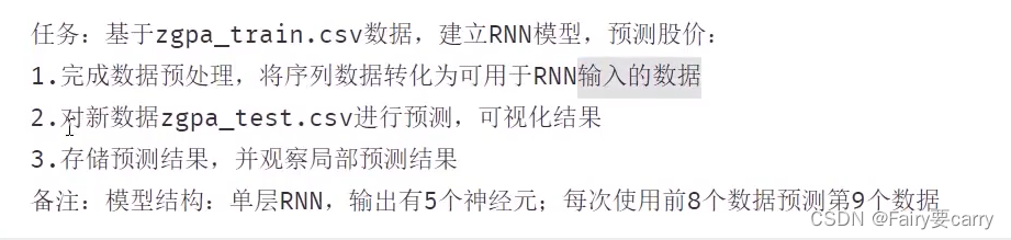
data = pd.read_csv('D:/pythonDATA/zgpa_train.csv')
print(data.head())

price = data.loc[:, 'close']
price.head()

# 归一化处理
price_norm = price / max(price)
print(price_norm)

from matplotlib import pyplot as plt

fig1 = plt.figure(figsize=(8, 5))
plt.plot(price)
plt.title('close price')
plt.xlabel('time')
plt.ylabel('price')
plt.show()


# define X and y
# define method to extract X and y
def extract_data(data, time_step):
    X = []
    y = []
    # 0,1,2...9:10个样本： time_step=8;0,1...7;1,2...8;2,3
    for i in range(len(data) - time_step):
        X.append([a for a in data[i:i + time_step]])
        y.append(data[i + time_step])
    X = np.array(X)
    # 723个数据，8个一步长，一维
    X = X.reshape(X.shape[0], X.shape[1], 1)
    return X, y


time_step = 8

# define X and y
X, y = extract_data(price_norm, time_step)
print("训练后的数据：")
print(X)
print(X.shape, len(y))
print("y的详细数据")
print(y)

# set up the model
from tensorflow.keras.models import Sequential
from tensorflow.keras.layers import Dense, SimpleRNN

model = Sequential()
# input_shape 训练长度 每个数据的维度
model.add(SimpleRNN(units=5, input_shape=(time_step, 1), activation="relu"))
# 输出层
# 输出数值 units =1 1个神经元 "linear"线性模型
model.add(Dense(units=1, activation="linear"))
# 配置模型 回归模型y
model.compile(optimizer="adam", loss="mean_squared_error")
model.summary()

y = np.array(y)

# train the model
model.fit(X, y, batch_size=30, epochs=200)

# make prediction based on the training data（model.predict(X)得到的是归一化的数据，所以需要*最大值）
y_train_predict = model.predict(X) * max(price)
y_train = y * max(price)
print("输出预测的数据")
print(y_train_predict, y_train)

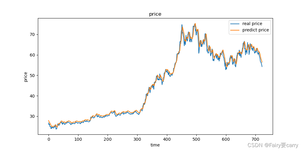
# 训练数据预测图
fig2 = plt.figure(figsize=(10, 5))
plt.plot(y_train, label="real price")
plt.plot(y_train_predict, label="predict price")
plt.title("price")
plt.xlabel("time")
plt.ylabel("price")
plt.legend()
plt.show()

# 基于测试数据的预测
data_test = pd.read_csv('D:/pythonDATA/zgpa_test.csv')
data_test.head()
price_test = data_test.loc[:, 'close']
price_test.head()
# 归一化
price_test_norm = price_test / max(price)
# extract X_test and y_test
X_test_norm, y_test_norm = extract_data(price_test_norm, time_step)
print("测试数据的纬度:")
print(X_test_norm.shape, len(y_test_norm))

# make prediction based on the test data（测试预测）
y_test_predict = model.predict(X_test_norm) * max(price)
y_test = [i * max(price) for i in y_test_norm]

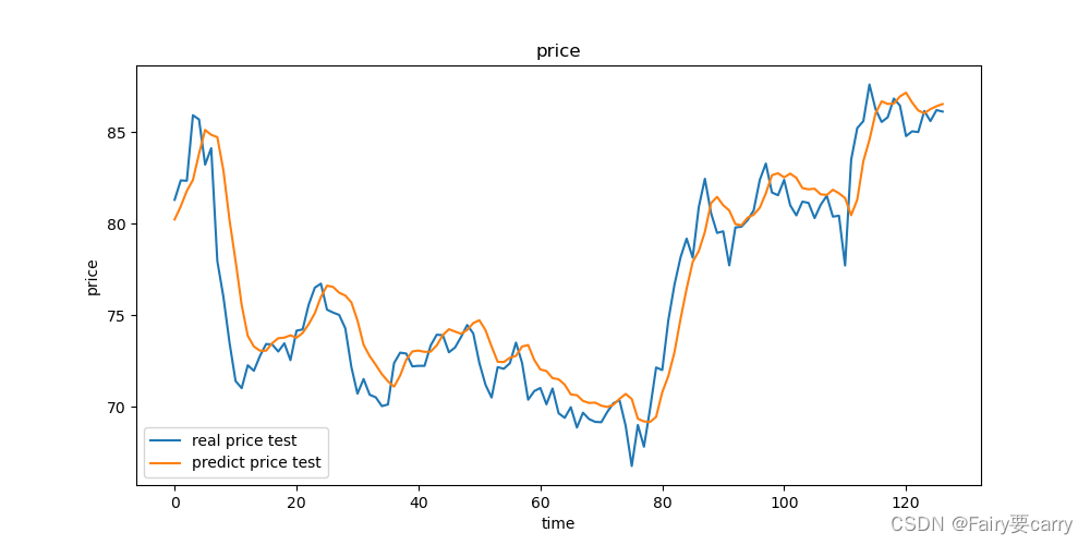
fig3 = plt.figure(figsize=(10, 5))
plt.plot(y_test, label="real price test")
plt.plot(y_test_predict, label="predict price test")
plt.title("price")
plt.xlabel("time")
plt.ylabel("price")
plt.legend()
plt.show()

# result_y_test = y_test.reshap(-1,1)
result_y_test = np.array(y_test).reshape(-1, 1)
result_y_test_predict = np.array(y_test_predict).reshape(-1, 1)
print(result_y_test.shape, result_y_test_predict.shape)
result = np.concatenate((result_y_test, result_y_test_predict), axis=1)
print(result.shape)
reslut = pd.DataFrame(result, columns=['real_price_test', 'predict_price_test'])
reslut.to_csv('zgpa_predict_test.csv')

训练集图：

基于测试集的图像：