pip install pmdarima
import numpy as np
import pandas as pd
import matplotlib.pyplot as plt
from pandas.plotting import lag_plot
from pandas.plotting import autocorrelation_plot
from datetime import date
from statsmodels.tsa.stattools import adfuller
from statsmodels.tsa.seasonal import seasonal_decompose
from statsmodels.tsa.arima.model import ARIMA
from sklearn.metrics import mean_squared_error
from pandas.plotting import register_matplotlib_converters
from pmdarima.arima import ADFTest
register_matplotlib_converters()
df = pd.read_csv('Tesla.csv')
print(df.head(5))
Date Open High Low Close Adj Close Volume
0 29/06/2010 1.266667 1.666667 1.169333 1.592667 1.592667 281494500
1 30/06/2010 1.719333 2.028000 1.553333 1.588667 1.588667 257806500
2 01/07/2010 1.666667 1.728000 1.351333 1.464000 1.464000 123282000
3 02/07/2010 1.533333 1.540000 1.247333 1.280000 1.280000 77097000
4 06/07/2010 1.333333 1.333333 1.055333 1.074000 1.074000 103003500
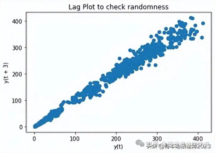
plt.figure()
lag_plot(df['Open'],lag=3)
plt.title('Lag Plot to check randomness')
plt.show
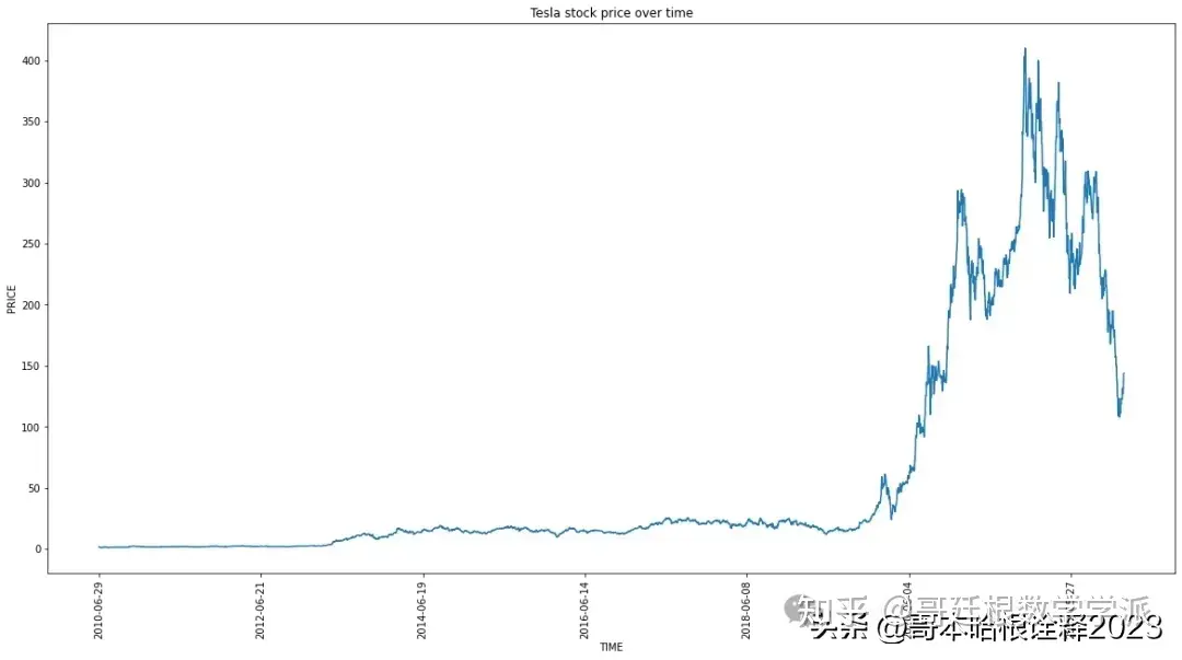
plt.figure(figsize=(20, 10))
plt.plot(df["Date"],df["Close"])
plt.xticks(np.arange(0,3500,500),df['Date'][0:3500:500],rotation='vertical')
plt.title("Tesla stock price over time")
plt.xlabel("TIME")
plt.ylabel("PRICE")
plt.show
adf_test=ADFTest(alpha = 0.05)
adf_test.should_diff(df['Close'])
result = seasonal_decompose(df["Close"],
                            model='multiplicative', period = 30)
fig = plt.figure()
fig = result.plot()
fig.set_size_inches(15, 10)

from statsmodels.tsa.stattools import adfuller
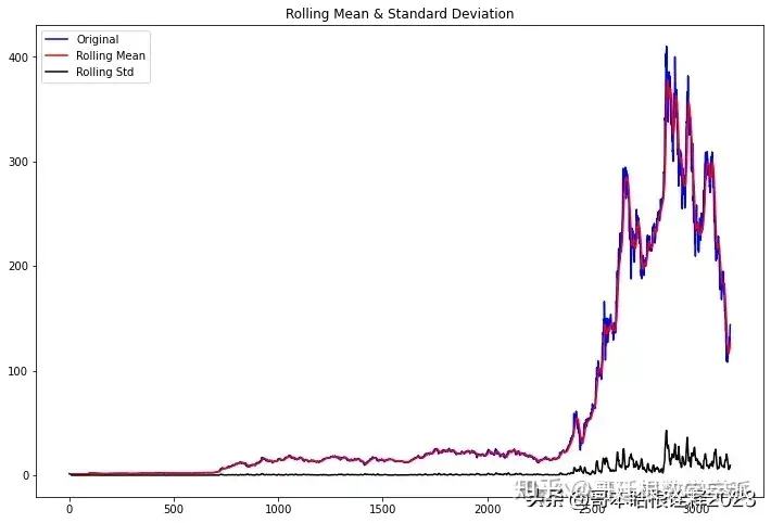
def test_stationarity(timeseries, window = 12):
#Determing rolling statistics
rolmean = timeseries.rolling(window).mean()
rolstd = timeseries.rolling(window).std()
#Plot rolling statistics:
fig = plt.figure(figsize=(12, 8))
orig = plt.plot(timeseries, color='blue',label='Original')
mean = plt.plot(rolmean, color='red', label='Rolling Mean')
std = plt.plot(rolstd, color='black', label = 'Rolling Std')
plt.legend(loc='best')
plt.title('Rolling Mean & Standard Deviation')
plt.show()
#Perform Dickey-Fuller test:
print('Results of Dickey-Fuller Test:')
dftest = adfuller(timeseries, autolag='AIC', maxlag = 20 )
dfoutput = pd.Series(dftest[0:4], index=['Test Statistic','p-value','#Lags Used','Number of Observations Used'])
for key,value in dftest[4].items():
dfoutput['Critical Value (%s)'%key] = value
pvalue = dftest[1]
if pvalue < 0.05:
print('p-value = %.4f. The series is likely stationary.' % pvalue)
else:
print('p-value = %.4f. The series is likely non-stationary.' % pvalue)
print(dfoutput)
test_stationarity(df['Close'])
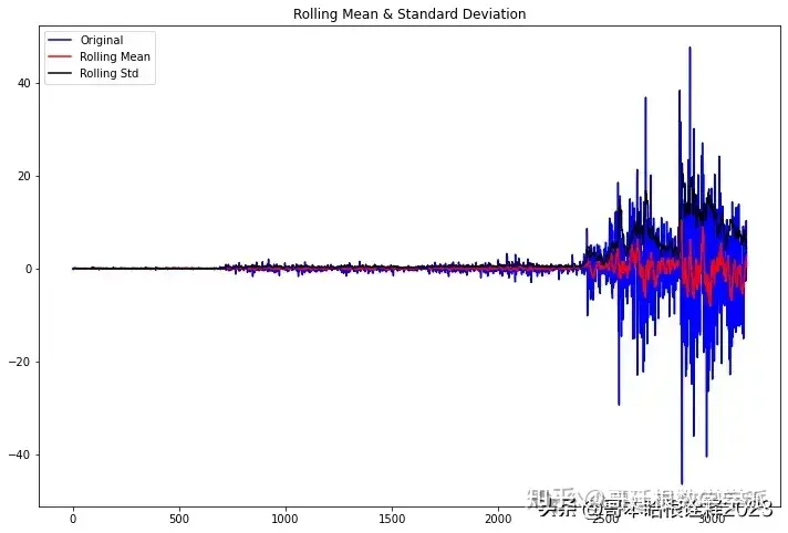
first_diff = df.Close - df.Close.shift(1)
first_diff = first_diff.dropna(inplace = False)
test_stationarity(first_diff, window = 12)
train_data, test_data = df[0:int(len(df)*0.7)], df[int(len(df)*0.7):]
training_data = train_data['Close'].values
test_data = test_data['Close'].values
history = [x for x in training_data]
model_predictions = []
N_test_observations = len(test_data)
for time_point in range(N_test_observations):
model = ARIMA(history, order=(4,1,0))
model_fit = model.fit()
output = model_fit.forecast()
yhat = output[0]
model_predictions.append(yhat)
true_test_value = test_data[time_point]
history.append(true_test_value)
MSE_error = mean_squared_error(test_data, model_predictions)
print('Testing Mean Squared Error is {}'.format(MSE_error))
print(model_fit.summary())
Testing Mean Squared Error is 66.13403523914238
SARIMAX Results
==============================================================================
Dep. Variable: y No. Observations: 3164
Model: ARIMA(4, 1, 0) Log Likelihood -9183.629
Date: Mon, 30 Jan 2023 AIC 18377.257
Time: 04:11:07 BIC 18407.554
Sample: 0 HQIC 18388.126
- 3164
Covariance Type: opg
==============================================================================
coef std err z P>|z| [0.025 0.975]
------------------------------------------------------------------------------
ar.L1 -0.0380 0.008 -4.899 0.000 -0.053 -0.023
ar.L2 0.0154 0.007 2.335 0.020 0.002 0.028
ar.L3 -0.0002 0.009 -0.024 0.981 -0.017 0.017
ar.L4 0.0407 0.007 5.747 0.000 0.027 0.055
sigma2 19.4734 0.136 143.711 0.000 19.208 19.739
===================================================================================
Ljung-Box (L1) (Q): 0.00 Jarque-Bera (JB): 80170.86
Prob(Q): 0.98 Prob(JB): 0.00
Heteroskedasticity (H): 1019.90 Skew: -0.15
Prob(H) (two-sided): 0.00 Kurtosis: 27.66
===================================================================================
Warnings:
[1] Covariance matrix calculated using the outer product of gradients (complex-step).
test_set_range = df[int(len(df)*0.7):].index
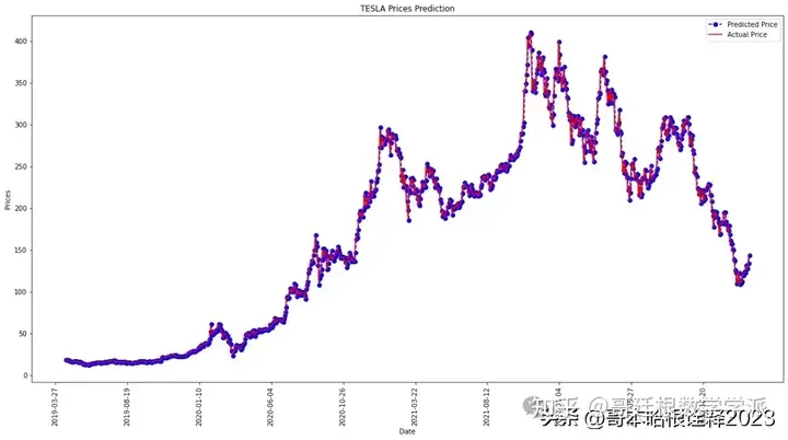
plt.figure(figsize=(20, 10))
plt.plot(test_set_range, model_predictions, color='blue', marker='o', linestyle='dashed',label='Predicted Price')
plt.plot(test_set_range, test_data, color='red', label='Actual Price')
plt.title('TESLA Prices Prediction')
plt.xlabel('Date')
plt.ylabel('Prices')
plt.xticks(np.arange(2200,3146,100), df.Date[2200:3146:100],rotation='vertical')
plt.legend()
plt.show()
担任《Mechanical System and Signal Processing》审稿专家,担任《中国电机工程学报》,《控制与决策》等EI期刊审稿专家,擅长领域:现代信号处理,机器学习,深度学习,数字孪生,时间序列分析,设备缺陷检测、设备异常检测、设备智能故障诊断与健康管理PHM等。

知乎学术咨询:https://www.zhihu.com/consult/people/792359672131756032?isMe=1