目录
前言
- 🍨 本文为🔗365天深度学习训练营中的学习记录博客
- 🍖 原作者:K同学啊
1.准备工作
import torch
import torch.nn as nn
import torchvision.transforms as transforms
import torchvision
from torchvision import transforms, datasets

import os,PIL,pathlib

device = torch.device("cuda" if torch.cuda.is_available() else "cpu")

device
2.查看数据
import os,PIL,random,pathlib

data_dir = 'data/45-data/'
data_dir = pathlib.Path(data_dir)

data_paths = list(data_dir.glob('*'))
classeNames = [str(path).split("\\")[2] for path in data_paths]
classeNames
3.划分数据集
total_datadir = 'data/45-data'

train_transforms = transforms.Compose([
    transforms.Resize([224, 224]),  # 将输入图片resize成统一尺寸
    transforms.ToTensor(),          # 将PIL Image或numpy.ndarray转换为tensor,并归一化到[0,1]之间
    transforms.Normalize(           # 标准化处理-->转换为标准正太分布(高斯分布),使模型更容易收敛
        mean=[0.485, 0.456, 0.406],
        std=[0.229, 0.224, 0.225])  # 其中 mean=[0.485,0.456,0.406]与std=[0.229,0.224,0.225] 从数据集中随机抽样计算得到的。
])

total_data = datasets.ImageFolder(total_datadir,transform=train_transforms)
total_data

train_size = int(0.8 * len(total_data))
test_size  = len(total_data) - train_size
train_dataset, test_dataset = torch.utils.data.random_split(total_data, [train_size, test_size])
train_dataset, test_dataset

train_size,test_size

batch_size = 32

train_dl = torch.utils.data.DataLoader(train_dataset,
                                           batch_size=batch_size,
                                           shuffle=True,
                                           num_workers=1)
test_dl = torch.utils.data.DataLoader(test_dataset,
                                          batch_size=batch_size,
                                          shuffle=True,
                                          num_workers=1)

for X, y in test_dl:
    print("Shape of X [N, C, H, W]: ", X.shape)
    print("Shape of y: ", y.shape, y.dtype)
    break
4.创建模型
 import torch
import torch.nn as nn
import torch.nn.functional as F

# SE注意力机制
class SqueezeExcitation(nn.Module):
    def __init__(self, in_channels, reduction=16):
        super(SqueezeExcitation, self).__init__()
        self.global_avg_pool = nn.AdaptiveAvgPool2d(1)
        self.fc1 = nn.Linear(in_channels, in_channels // reduction, bias=False)
        self.relu = nn.ReLU(inplace=True)
        self.fc2 = nn.Linear(in_channels // reduction, in_channels, bias=False)
        self.sigmoid = nn.Sigmoid()

    def forward(self, x):
        b, c, _, _ = x.size()
        y = self.global_avg_pool(x).view(b, c)
        y = self.fc1(y)
        y = self.relu(y)
        y = self.fc2(y)
        y = self.sigmoid(y).view(b, c, 1, 1)
        return x * y

# DenseNet的Conv Block
class ConvBlock(nn.Module):
    def __init__(self, in_channels, growth_rate):
        super(ConvBlock, self).__init__()
        self.bn1 = nn.BatchNorm2d(in_channels)
        self.relu = nn.ReLU(inplace=True)
        self.conv1 = nn.Conv2d(in_channels, 4 * growth_rate, kernel_size=1, bias=False)
        self.bn2 = nn.BatchNorm2d(4 * growth_rate)
        self.conv2 = nn.Conv2d(4 * growth_rate, growth_rate, kernel_size=3, padding=1, bias=False)

    def forward(self, x):
        out = self.conv1(self.relu(self.bn1(x)))
        out = self.conv2(self.relu(self.bn2(out)))
        return torch.cat([x, out], 1)

# Dense Block
class DenseBlock(nn.Module):
    def __init__(self, num_layers, in_channels, growth_rate):
        super(DenseBlock, self).__init__()
        layers = []
        for i in range(num_layers):
            layers.append(ConvBlock(in_channels + i * growth_rate, growth_rate))
        self.block = nn.Sequential(*layers)

    def forward(self, x):
        return self.block(x)

# Transition Block
class TransitionBlock(nn.Module):
    def __init__(self, in_channels, out_channels):
        super(TransitionBlock, self).__init__()
        self.bn = nn.BatchNorm2d(in_channels)
        self.relu = nn.ReLU(inplace=True)
        self.conv = nn.Conv2d(in_channels, out_channels, kernel_size=1, bias=False)
        self.pool = nn.AvgPool2d(kernel_size=2, stride=2)

    def forward(self, x):
        x = self.conv(self.relu(self.bn(x)))
        x = self.pool(x)
        return x

# DenseNet
class DenseNet(nn.Module):
    def __init__(self, growth_rate=32, block_config=(6, 12, 24, 16), num_init_features=64, num_classes=3):
        super(DenseNet, self).__init__()

        # 初始卷积层
        self.features = nn.Sequential(
            nn.Conv2d(3, num_init_features, kernel_size=7, stride=2, padding=3, bias=False),
            nn.BatchNorm2d(num_init_features),
            nn.ReLU(inplace=True),
            nn.MaxPool2d(kernel_size=3, stride=2, padding=1)
        )

        num_features = num_init_features
        layers = []
        for i, num_layers in enumerate(block_config):
            layers.append(DenseBlock(num_layers, num_features, growth_rate))
            num_features += num_layers * growth_rate
            if i != len(block_config) - 1:
                layers.append(TransitionBlock(num_features, num_features // 2))
                num_features = num_features // 2

        self.dense_blocks = nn.Sequential(*layers)
        self.se = SqueezeExcitation(num_features)
        self.final_bn = nn.BatchNorm2d(num_features)
        self.final_relu = nn.ReLU(inplace=True)
        self.global_avg_pool = nn.AdaptiveAvgPool2d(1)
        self.classifier = nn.Linear(num_features, num_classes)

    def forward(self, x):
        x = self.features(x)
        x = self.dense_blocks(x)
        x = self.se(x)
        x = self.final_relu(self.final_bn(x))
        x = self.global_avg_pool(x)
        x = torch.flatten(x, 1)
        x = self.classifier(x)
        return x

# 定义不同版本的 DenseNet

def densenet121(num_classes=3):
    return DenseNet(growth_rate=32, block_config=(6, 12, 24, 16), num_init_features=64, num_classes=num_classes)

def densenet169(num_classes=3):
    return DenseNet(growth_rate=32, block_config=(6, 12, 32, 32), num_init_features=64, num_classes=num_classes)

def densenet201(num_classes=3):
    return DenseNet(growth_rate=32, block_config=(6, 12, 48, 32), num_init_features=64, num_classes=num_classes)

model=densenet121().to(device)
model
5.编译及训练模型
loss_fn    = nn.CrossEntropyLoss() # 创建损失函数
learn_rate = 1e-4 # 学习率
opt        = torch.optim.SGD(model.parameters(),lr=learn_rate)

# 训练循环
def train(dataloader, model, loss_fn, optimizer):
    size = len(dataloader.dataset)  # 训练集的大小,一共60000张图片
    num_batches = len(dataloader)   # 批次数目,1875(60000/32)

    train_loss, train_acc = 0, 0  # 初始化训练损失和正确率

    for X, y in dataloader:  # 获取图片及其标签
        X, y = X.to(device), y.to(device)

        # 计算预测误差
        pred = model(X)          # 网络输出
        loss = loss_fn(pred, y)  # 计算网络输出和真实值之间的差距,targets为真实值,计算二者差值即为损失

        # 反向传播
        optimizer.zero_grad()  # grad属性归零
        loss.backward()        # 反向传播
        optimizer.step()       # 每一步自动更新

        # 记录acc与loss
        train_acc  += (pred.argmax(1) == y).type(torch.float).sum().item()
        train_loss += loss.item()

    train_acc  /= size
    train_loss /= num_batches

    return train_acc, train_loss

def test (dataloader, model, loss_fn):
    size        = len(dataloader.dataset)  # 测试集的大小,一共10000张图片
    num_batches = len(dataloader)          # 批次数目,313(10000/32=312.5,向上取整)
    test_loss, test_acc = 0, 0

    # 当不进行训练时,停止梯度更新,节省计算内存消耗
    with torch.no_grad():
        for imgs, target in dataloader:
            imgs, target = imgs.to(device), target.to(device)

            # 计算loss
            target_pred = model(imgs)
            loss        = loss_fn(target_pred, target)

            test_loss += loss.item()
            test_acc  += (target_pred.argmax(1) == target).type(torch.float).sum().item()

    test_acc  /= size
    test_loss /= num_batches

    return test_acc, test_loss

epochs     = 20
train_loss = []
train_acc  = []
test_loss  = []
test_acc   = []

for epoch in range(epochs):
    model.train()
    epoch_train_acc, epoch_train_loss = train(train_dl, model, loss_fn, opt)

    model.eval()
    epoch_test_acc, epoch_test_loss = test(test_dl, model, loss_fn)

    train_acc.append(epoch_train_acc)
    train_loss.append(epoch_train_loss)
    test_acc.append(epoch_test_acc)
    test_loss.append(epoch_test_loss)

    template = ('Epoch:{:2d}, Train_acc:{:.1f}%, Train_loss:{:.3f}, Test_acc:{:.1f}%,Test_loss:{:.3f}')
    print(template.format(epoch+1, epoch_train_acc*100, epoch_train_loss, epoch_test_acc*100, epoch_test_loss))
print('Done')
6.结果可视化
import matplotlib.pyplot as plt
#隐藏警告
import warnings
warnings.filterwarnings("ignore")               #忽略警告信息
plt.rcParams['font.sans-serif']    = ['SimHei'] # 用来正常显示中文标签
plt.rcParams['axes.unicode_minus'] = False      # 用来正常显示负号
plt.rcParams['figure.dpi']         = 100        #分辨率

from datetime import datetime
current_time = datetime.now() # 获取当前时间

epochs_range = range(epochs)

plt.figure(figsize=(12, 3))
plt.subplot(1, 2, 1)

plt.plot(epochs_range, train_acc, label='Training Accuracy')
plt.plot(epochs_range, test_acc, label='Test Accuracy')
plt.legend(loc='lower right')
plt.title('Training and Validation Accuracy')
plt.xlabel(current_time) # 打卡请带上时间戳,否则代码截图无效

plt.subplot(1, 2, 2)
plt.plot(epochs_range, train_loss, label='Training Loss')
plt.plot(epochs_range, test_loss, label='Test Loss')
plt.legend(loc='upper right')
plt.title('Training and Validation Loss')
plt.show()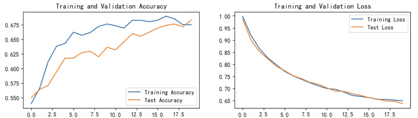
7.总结
在本次尝试中,我将SE(Squeeze-and-Excitation)模块集成到了DenseNet架构之中,以进一步增强网络对通道维度信息的建模能力。DenseNet以其密集连接的特性而闻名,每一层都会接收前面所有层的特征图输入,这种结构极大地促进了特征重用与梯度传播。而SE模块则专注于通过显式建模通道间的依赖关系,动态地为每个通道分配权重,从而提升网络对关键特征的关注能力。
在实现过程中,我将SE模块插入到每个DenseLayer之后,使得每一小层都具备一定的通道注意力调节能力。具体来说,每个DenseLayer输出的特征图会先经过SE模块处理,再被传入后续连接中。这种策略保持了DenseNet原有的特征级联路径,同时也在更微观的层面上增强了特征表达能力。
SE模块的实现相对简单,主要包括三个步骤:首先通过全局平均池化将空间信息压缩为通道描述向量;然后通过两个全连接层(中间通常加入ReLU激活)构建非线性的通道间关系;最后使用Sigmoid函数将输出归一化为0到1之间的权重,重新作用于输入特征图的通道维度上。这里我采用了标准的reduction ratio = 16,以在参数量和表现之间取得平衡。
值得注意的是,DenseNet本身已经具备一定的信息融合能力,加入SE模块后所带来的性能提升虽不如在ResNet中那般显著,但在若干分类任务中仍可观察到精度的稳定上升。同时,由于SE模块引入了额外的计算量,在参数量与推理时间上也有一定代价,但整体在可接受范围之内。
这种融合策略体现了一种“通道敏感 + 特征重用”的设计理念,也为后续尝试更多类型的注意力机制(如CBAM、ECA)埋下了基础。在未来工作中,我也希望进一步探索SE模块在DenseNet-B、DenseNet-C等改进版本中的兼容性与性能表现。