- 🍨 本文为🔗365天深度学习训练营中的学习记录博客
- 🍖 原作者:
一、前期准备
1.导入数据
import pandas as pd
import numpy as np

df_1 = pd.read_csv("D:\TensorFlow1\woodpine2.csv")
df_1

import matplotlib.pyplot as plt
import seaborn as sns

plt.rcParams['savefig.dpi'] = 500 #图片像素
plt.rcParams['figure.dpi']  = 500 #分辨率

fig, ax =plt.subplots(1,3,constrained_layout=True, figsize=(14, 3))

sns.lineplot(data=df_1["Tem1"], ax=ax[0])
sns.lineplot(data=df_1["CO 1"], ax=ax[1])
sns.lineplot(data=df_1["Soot 1"], ax=ax[2])
plt.show()

dataFrame = df_1.iloc[:,1:]
dataFrame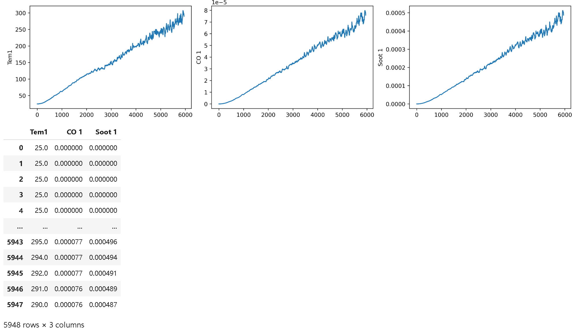
 编辑2.划分数据集
width_X = 8
width_y = 1

X = []
y = []

in_start = 0

for _, _ in df_1.iterrows():
    in_end  = in_start + width_X
    out_end = in_end   + width_y

    if out_end < len(dataFrame):
        X_ = np.array(dataFrame.iloc[in_start:in_end , ])
        X_ = X_.reshape((len(X_)*3))
        y_ = np.array(dataFrame.iloc[in_end  :out_end, 0])

        X.append(X_)
        y.append(y_)

    in_start += 1

X = np.array(X)
y = np.array(y)

X.shape, y.shape

from sklearn.preprocessing import MinMaxScaler

#将数据归一化,范围是0到1
sc       = MinMaxScaler(feature_range=(0, 1))
X_scaled = sc.fit_transform(X)
X_scaled.shape

X_scaled = X_scaled.reshape(len(X_scaled),width_X,3)
X_scaled.shape

X_train = np.array(X_scaled[:5000]).astype('float64')
y_train = np.array(y[:5000]).astype('float64')

X_test  = np.array(X_scaled[5000:]).astype('float64')
y_test  = np.array(y[5000:]).astype('float64')

X_train.shape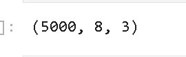
二、构建模型
from tensorflow.keras.models import Sequential
from tensorflow.keras.layers import Dense,LSTM,Bidirectional
from tensorflow.keras        import Input

# 多层 LSTM
model_lstm = Sequential()
model_lstm.add(LSTM(units=64, activation='relu', return_sequences=True,
               input_shape=(X_train.shape[1], 3)))
model_lstm.add(LSTM(units=64, activation='relu'))

model_lstm.add(Dense(width_y))
三、编译模型
# 只观测loss数值,不观测准确率,所以删去metrics选项
import tensorflow as tf
model_lstm.compile(optimizer=tf.keras.optimizers.Adam(1e-3),
                   loss='mean_squared_error')  # 损失函数用均方误差
四、训练模型
history_lstm = model_lstm.fit(X_train, y_train,
                         batch_size=64,
                         epochs=40,
                         validation_data=(X_test, y_test),
                         validation_freq=1)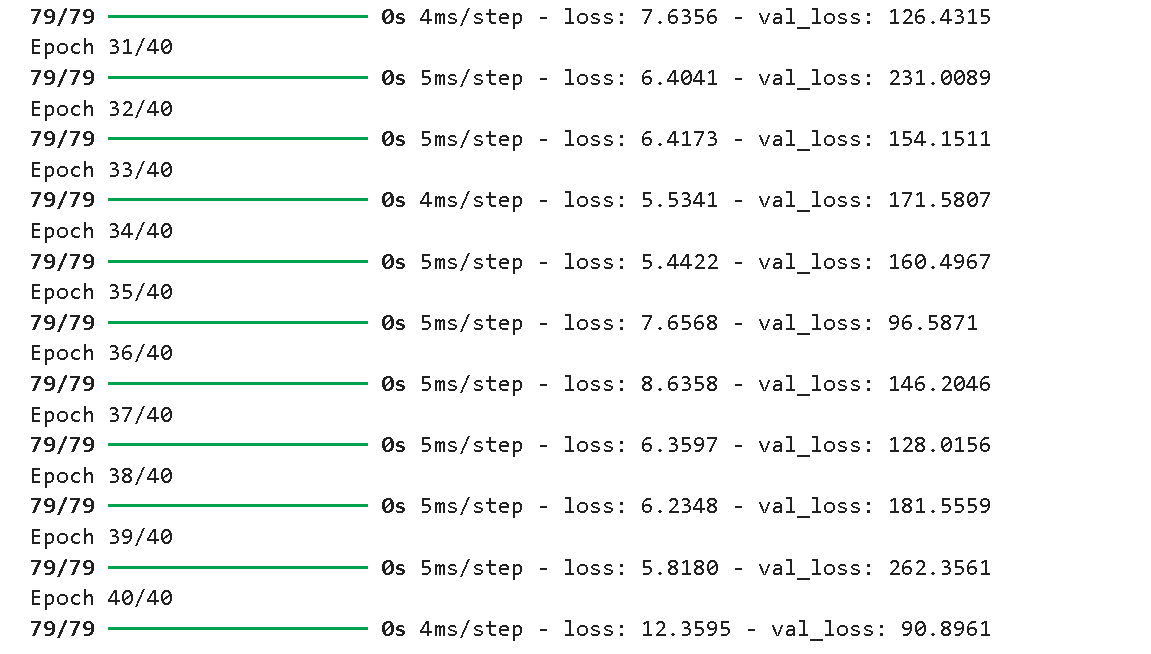
五、模型评估及可视化
# 支持中文
plt.rcParams['font.sans-serif'] = ['SimHei']  # 用来正常显示中文标签
plt.rcParams['axes.unicode_minus'] = False  # 用来正常显示负号

plt.figure(figsize=(5, 3),dpi=120)

plt.plot(history_lstm.history['loss']    , label='LSTM Training Loss')
plt.plot(history_lstm.history['val_loss'], label='LSTM Validation Loss')

plt.title('Training and Validation Loss')
plt.legend()
plt.show()

predicted_y_lstm = model_lstm.predict(X_test)                        # 测试集输入模型进行预测

y_test_one = [i[0] for i in y_test]
predicted_y_lstm_one = [i[0] for i in predicted_y_lstm]

plt.figure(figsize=(5, 3),dpi=120)
# 画出真实数据和预测数据的对比曲线
plt.plot(y_test_one[:1000], color='red', label='真实值')
plt.plot(predicted_y_lstm_one[:1000], color='blue', label='预测值')

plt.title('Title')
plt.xlabel('X')
plt.ylabel('Y')
plt.legend()
plt.show() 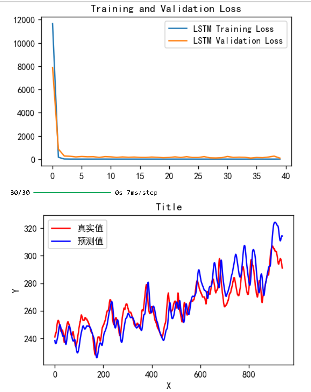
from sklearn import metrics
RMSE_lstm=metrics.mean_squared_error(predicted_y_lstm,y_test)**0.5
R2_lstm=metrics.r2_score(predicted_y_lstm,y_test)
print("均方误差:%.5f" %RMSE_lstm)
print("R2:%.5f" %R2_lstm)
六、总结
数据探索与预处理
- 数据结构:数据集包含 5948 条记录,特征列为 Time、Tem1、CO1、Soot1,其中 Time 为时间戳,Tem1 为目标变量。
- 可视化分析:使用
matplotlib和seaborn绘制时间序列曲线,观察到 Tem1 在后期显著上升(最高达 295℃),CO1 和 Soot1 呈缓慢增长趋势,初步判断数据具备时间依赖特征。 - 归一化处理:通过
MinMaxScaler将特征值缩放到 [0, 1] 区间,确保模型收敛稳定性。 - 滑动窗口构造样本:采用宽度为 8 的滑动窗口生成输入特征 X(包含连续 8 个时间步的 3 个特征),目标值 y 为第 9 个时间步的 Tem1,最终形成形状为
(样本数, 8, 3)的输入数据。
LSTM 模型构建
- 网络架构:
- 第一层:双向 LSTM 层,64 个隐藏单元,激活函数 ReLU,返回序列以支持后续 LSTM 层。
- 第二层:单向 LSTM 层,64 个隐藏单元,提取高层时间特征。
- 输出层:全连接层,单神经元,直接输出预测温度值。
- 编译配置:使用均方误差(MSE)作为损失函数,Adam 优化器(学习率 1e-3),聚焦回归任务的误差优化。
- 网络架构:
模型训练与验证
- 数据集划分:前 5000 条样本为训练集,剩余 939 条为测试集。
- 训练参数:批量大小 64,训练 40 个 epoch,每 epoch 后使用测试集验证(
validation_freq=1)。 - 训练结果:
- 训练损失稳定在 5-8 之间,但验证损失波动较大,可能存在过拟合或数据分布不均问题。
结果可视化与评估
- 损失曲线:训练损失与验证损失趋势基本一致,但验证损失整体高于训练损失,表明模型泛化能力有待提升。
- 预测对比:真实值与预测值的前 1000 个样本曲线显示,模型在趋势变化(如温度上升)时能捕捉大致走向,但在细节波动上存在偏差。
- 定量指标:
- 均方根误差(RMSE):9.53,反映预测值与真实值的平均偏差。
- 决定系数(R²):0.82162,表明模型解释了 82.162% 的目标变量变化,拟合效果中等偏上。