本文是实验设计与分析(第6版,Montgomery著,傅珏生译) 第5章析因设计引导5.7节思考题5.6 R语言解题。主要涉及方差分析,正态假设检验,残差分析,交互作用图,等值线图。
dataframe <-data.frame(
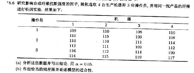
strength=c(109,110,110,112,116,114,110,115,110,111,112,115,108,109,111,109,114,119,110,108,114,112,120,117),
machine=gl(4,6,24),
operator=gl(3,2,24))
summary (dataframe)
dataframe.aov2 <- aov(strength~operator*machine,data=dataframe)
summary (dataframe.aov2)
> summary (dataframe.aov2)
Df Sum Sq Mean Sq F value Pr(>F)
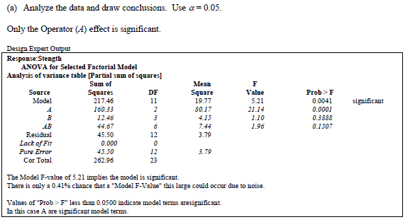
operator 2 160.33 80.17 21.143 0.000117 ***
machine 3 12.46 4.15 1.095 0.388753
operator:machine 6 44.67 7.44 1.963 0.150681
Residuals 12 45.50 3.79
---
Signif. codes: 0 ‘***’ 0.001 ‘**’ 0.01 ‘*’ 0.05 ‘.’ 0.1 ‘ ’ 1
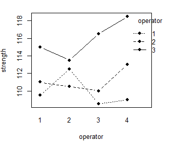
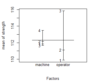
with(dataframe,interaction.plot(machine,operator,strength,type="b",pch=19,fixed=T,xlab="operator",ylab="strength"))
plot.design(strength~machine*operator,data=dataframe)
fit <-lm(strength~operator*machine,data=dataframe)
anova(fit)
> anova(fit)
Analysis of Variance Table
Response: strength
Df Sum Sq Mean Sq F value Pr(>F)
operator 2 160.333 80.167 21.1429 0.0001167 ***
machine 3 12.458 4.153 1.0952 0.3887526
operator:machine 6 44.667 7.444 1.9634 0.1506807
Residuals 12 45.500 3.792
---
Signif. codes: 0 ‘***’ 0.001 ‘**’ 0.01 ‘*’ 0.05 ‘.’ 0.1 ‘ ’ 1
summary(fit)
> summary(fit)
Call:
lm(formula = strength ~ operator * machine, data = dataframe)
Residuals:
Min 1Q Median 3Q Max
-2.5 -1.0 0.0 1.0 2.5
Coefficients:
Estimate Std. Error t value Pr(>|t|)
(Intercept) 1.095e+02 1.377e+00 79.527 <2e-16 ***
operator2 1.500e+00 1.947e+00 0.770 0.4560
operator3 5.500e+00 1.947e+00 2.825 0.0153 *
machine2 3.000e+00 1.947e+00 1.541 0.1493
machine3 -1.000e+00 1.947e+00 -0.514 0.6169
machine4 -5.000e-01 1.947e+00 -0.257 0.8017
operator2:machine2 -3.500e+00 2.754e+00 -1.271 0.2278
operator3:machine2 -4.500e+00 2.754e+00 -1.634 0.1282
operator2:machine3 8.808e-14 2.754e+00 0.000 1.0000
operator3:machine3 2.500e+00 2.754e+00 0.908 0.3818
operator2:machine4 2.500e+00 2.754e+00 0.908 0.3818
operator3:machine4 4.000e+00 2.754e+00 1.453 0.1720
---
Signif. codes: 0 ‘***’ 0.001 ‘**’ 0.01 ‘*’ 0.05 ‘.’ 0.1 ‘ ’ 1
Residual standard error: 1.947 on 12 degrees of freedom
Multiple R-squared: 0.827, Adjusted R-squared: 0.6684
F-statistic: 5.214 on 11 and 12 DF, p-value: 0.004136
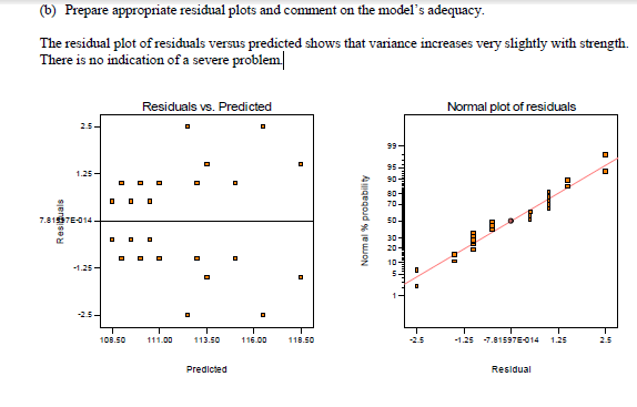
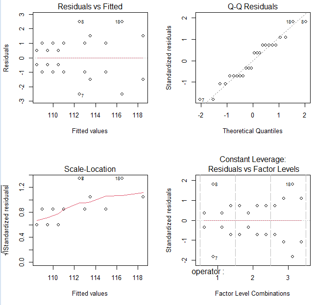
par(mfrow=c(2,2))
plot(fit)
par(mfrow=c(2,2))
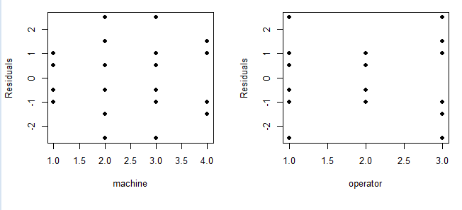
plot(as.numeric(dataframe$machine), fit$residuals, xlab="machine", ylab="Residuals", type="p", pch=16)
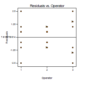
plot(as.numeric(dataframe$operator), fit$residuals, xlab="operator", ylab="Residuals", pch=16)