本文为🔗365天深度学习训练营内部文章
原作者:K同学啊
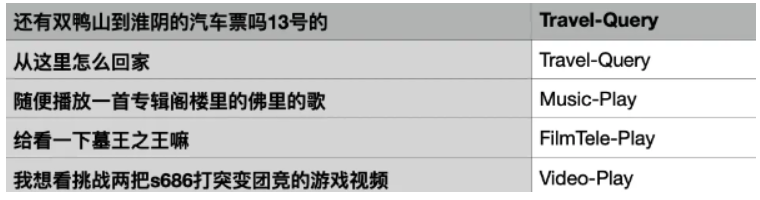
本次将加入Word2vec使用PyTorch实现中文文本分类,Word2Vec 则是其中的一种词嵌入方法,是一种用于生成词向量的浅层神经网络模型,由Tomas Mikolov及其团队于2013年提出。Word2Vec通过学习大量文本数据,将每个单词表示为一个连续的向量,这些向量可以捕捉单词之间的语义和句法关系。数据示例如下:
1.加载数据
import time
import pandas as pd
import torch
from torch.utils.data import DataLoader, random_split
import torch.nn as nn
import torchvision
from torchtext.data import to_map_style_dataset
from torchvision import transforms,datasets
from torchtext.data.utils import get_tokenizer
from torchtext.vocab import build_vocab_from_iterator
from gensim.models.word2vec import Word2Vec
import numpy as np
import jieba
import warnings

warnings.filterwarnings('ignore')
device = torch.device("cuda" if torch.cuda.is_available() else "cpu")

'''
加载本地数据
'''
train_data = pd.read_csv('train.csv',sep='\t',header=None)
print(train_data.head())
# 构建数据集迭代器
def coustom_data_iter(texts,labels):
    for x,y in zip(texts,labels):
        yield x,y

x = train_data[0].values[:]
y = train_data[1].values[:]
zip 是 Python 中的一个内置函数,它可以将多个序列(列表、元组等)中对应的元素打包,成一个个元组,然后返回这些元组组成的一个迭代器。例如,在代码中 zip(texts,labels)就是将 texts 和labels 两个列表中对应位置的元素一一打包,成元组,返回一个迭代器,每次迭代返回一个元组(x,y)其中x是 texts 中的一个元素,y是 labels 中对应的一个元素。这样,每次从迭代器中获取一个元素,就相当于从 texts 和 labels 中获取了一组对应的数据。在这里,zip 函数主要用于将输入的 texts 和labels打包成一个可迭代的数据集,然后传给后续的模型训练过程使用。
2.数据预处理
1)构建词典
# 1.构建词典
# 训练 Word2Vec 浅层神经网络模型
w2v = Word2Vec(vector_size=100,   # 是指特征向量的维度,默认为100
               min_count=3)  # 可以对字典做截断,词频少于min_count次数的单词会被丢弃掉,默认为5
w2v.build_vocab(x)
w2v.train(x,total_examples=w2v.corpus_count,epochs=20)
Word2Vec可以直接训练模型,一步到位。这里分了三步 第一步构建一个空模型 第二步使用 build_vocab 方法根据输入的文本数据x构建词典。build_vocab 方法会统计输入文本中每个词汇出现的次数,并按照词频从高到低的顺序将词汇加入词典中。 第三步使用 train 方法对模型进行训练,total_examples 参数指定了训练时使用的文本数量,这里使用的是 w2v.corpus_count 属性,表示输入文本的数量
# 将文本转化为向量
def average_vec(text):
    vec = np.zeros(100).reshape((1,100))
    for word in text:
        try:
            vec += w2v.wv[word].reshape((1,100))
        except KeyError:
            continue
    return vec

# 将词向量保存为Ndarray
x_vec = np.concatenate([average_vec(z) for z in x])

# 保存word2vec模型和词向量
w2v.save('w2v_model.pkl')
这段代码定义了一个函数 average_vec(text),它接受一个包含多个词的列表 text 作为输入,并返回这些词对应词向量的平均值。该函数 首先初始化一个形状为(1,100)的全零 numpy 数组来表示平均向量 然后遍历 text 中的每个词,并尝试从 Word2Vec 模型 w2v 中使用 wv 属性获取其对应的词向量。如果在模型中找到了该词,函数将其向量加到 vec 中。如果未找到该词,函数会继续迭代下一个词 最后,函数返回平均向量 vec 然后使用列表推导式将 average_vec()函数应用于列表x中的每个元素。得到的平均向量列表使用 np.concatenate()连接成一个numpy数组x vec,该数组表示x中所有元素的平均向量。x vec的形状为(n,18),其中n是x中元素的数量。
train_iter = coustom_data_iter(x_vec,y)
print(len(x),len(x_vec))
label_name = list(set(train_data[1].values[:]))
print(label_name)

text_pipeline = lambda x:average_vec(x)
label_pipeline = lambda x:label_name.index(x)
lambda 表达式的语法为:lambda arguments:expression 其中 arguments 是函数的参数,可以有多个参数,用逗号分隔。expression 是一个表达式,它定义了函数的返回值。 text_pipeline函数:将原始文本数据转换为整数列表,使用了之前构建的vocab词表和tokenizer分词器函数。具体来说,它接受一个字符串x作为输入,首先使用tokenizer将其分词,然后将每个词在vocab词表中的索引放入一个列表中返回。 label pipeline函数:将原始标签数据转换为整数,它接受一个字符串x作为输入,并使用 label_name.index(x)方法获取x在label name 列表中的索引作为输出。
2)生成数据批次和迭代器
# 2.生成数据批次和迭代器
def collate_batch(batch):
    label_list,text_list = [],[]

    for (_text,_label) in batch:
        # 标签列表
        label_list.append(label_pipeline(_label))

        # 文本列表
        processed_text = torch.tensor(text_pipeline(_text),dtype=torch.float32)
        text_list.append(processed_text)

    label_list = torch.tensor(label_list,dtype=torch.int64)
    text_list = torch.cat(text_list)

    return text_list.to(device),label_list.to(device)

# 数据加载器
dataloader = DataLoader(train_iter,batch_size=8,shuffle=False,collate_fn=collate_batch)
3.构建模型
由于这次我们使用了Word2Vec方法构建词向量作为词嵌入的方法,因此这次的模型不需要嵌入层。选取最简单的模
# 1.定义模型(此时不需要嵌入层了)
class TextClassificationModel(nn.Module):
    def __init__(self,num_class):
        super(TextClassificationModel,self).__init__()
        self.fc = nn.Linear(100,num_class)

    def forward(self,text):
        return self.fc(text)

# 2.定义实例
num_class = len(label_name)
vocab_size = 100000
em_size = 12
model = TextClassificationModel(num_class).to(device)

# 3.定义训练函数和评估函数
def train(dataloader):
    model.train()
    total_acc,train_loss,total_count = 0,0,0
    log_interval = 50
    start_time = time.time()

    for idx,(text,label) in enumerate(dataloader):
        predicted_label = model(text)
        optimzer.zero_grad()   # grad属性归零
        loss = criterion(predicted_label,label)   # 计算网络输出和真实值之间的差距
        loss.backward()   # 反向传播
        nn.utils.clip_grad_norm(model.parameters(),0.1)   # 梯度裁剪
        optimzer.step()  # 每一步自动更新

        # 记录acc与Loss
        total_acc += (predicted_label.argmax(1) == label).sum().item()
        train_loss += loss.item()
        total_count += label.size(0)

        if idx % log_interval == 0 and idx > 0:
            elapsed = time.time() - start_time
            print('| epoch {:1d} | {:4d}/{:4d} batches '
                  '| train_acc {:4.3f} train_loss {:4.5f}'.format(epoch,idx,len(dataloader),
                                                                  total_acc/total_count,train_loss/total_count))
            total_acc,train_loss,total_count = 0,0,0
            start_time = time.time()

def evaluate(dataloader):
    model.eval()
    total_acc, train_loss, total_count = 0, 0, 0

    with torch.no_grad():
        for idx, (text,label) in enumerate(dataloader):
            predicted_label = model(text)
            loss = criterion(predicted_label, label)  # 计算网络输出和真实值之间的差距

            # 记录acc与Loss
            total_acc += (predicted_label.argmax(1) == label).sum().item()
            train_loss += loss.item()
            total_count += label.size(0)
    return total_acc/total_count,train_loss/total_count
4.训练模型
# 1.拆分数据集并运行模型
EPOCHS = 10
LR = 5
BATCH_SIZE = 64

criterion = torch.nn.CrossEntropyLoss()
optimzer = torch.optim.SGD(model.parameters(),lr=LR)
scheduler = torch.optim.lr_scheduler.StepLR(optimzer,1.0,gamma=0.1)
total_accu = None

# 构建数据集
train_iter = coustom_data_iter(train_data[0].values[:],train_data[1].values[:])
train_dataset = to_map_style_dataset(train_iter)
split_train_,split_valid_ = random_split(train_dataset,[int(len(train_dataset)*0.8),int(len(train_dataset)*0.2)])
train_dataloader = DataLoader(split_train_,batch_size=BATCH_SIZE,shuffle=True,collate_fn=collate_batch)
valid_dataloader = DataLoader(split_valid_,batch_size=BATCH_SIZE,shuffle=True,collate_fn=collate_batch)

for epoch in range(1,EPOCHS+1):
    epoch_start_time = time.time()
    train(train_dataloader)
    val_acc,val_loss = evaluate(valid_dataloader)

    # 获取当前的学习率
    lr = optimzer.state_dict()['param_groups'][0]['lr']

    if total_accu is not None and total_accu > val_acc:
        scheduler.step()
    else:
        total_accu = val_acc
    print('-'*69)
    print('| epoch {:1d} | time:{:4.2f}s | '
          'valid_acc {:4.3f} valid_loss {:4.3f}'.format(epoch,time.time()-epoch_start_time,val_acc,val_loss))
    print('-'*69)

# 2.使用测试数据集评估模型
print('Checking the results of test dataset.')
test_acc,test_loss = evaluate(valid_dataloader)
print('test accuracy {:8.3f}'.format(test_acc))

# 3.测试指定数据
def predict(text,text_pipeline):
    with torch.no_grad():
        text = torch.tensor(text_pipeline(text),dtype=torch.float32)
        print(text.shape)
        output = model(text)
        return output.argmax(1).item()

ex_text = "开始打王者荣耀啦"
model = model.to("cpu")
print('该文本的类别是:%s'%label_name[predict(ex_text,text_pipeline)])
| epoch 1 | 50/ 152 batches | train_acc 0.733 train_loss 0.02502 | epoch 1 | 100/ 152 batches | train_acc 0.831 train_loss 0.01846 | epoch 1 | 150/ 152 batches | train_acc 0.827 train_loss 0.01916 --------------------------------------------------------------------- | epoch 1 | time:0.88s | valid_acc 0.828 valid_loss 0.022 --------------------------------------------------------------------- | epoch 2 | 50/ 152 batches | train_acc 0.829 train_loss 0.01900 | epoch 2 | 100/ 152 batches | train_acc 0.844 train_loss 0.01736 | epoch 2 | 150/ 152 batches | train_acc 0.847 train_loss 0.01747 --------------------------------------------------------------------- | epoch 2 | time:0.91s | valid_acc 0.827 valid_loss 0.019 --------------------------------------------------------------------- | epoch 3 | 50/ 152 batches | train_acc 0.879 train_loss 0.00987 | epoch 3 | 100/ 152 batches | train_acc 0.900 train_loss 0.00786 | epoch 3 | 150/ 152 batches | train_acc 0.892 train_loss 0.00829 --------------------------------------------------------------------- | epoch 3 | time:0.92s | valid_acc 0.876 valid_loss 0.011 --------------------------------------------------------------------- | epoch 4 | 50/ 152 batches | train_acc 0.904 train_loss 0.00655 | epoch 4 | 100/ 152 batches | train_acc 0.903 train_loss 0.00710 | epoch 4 | 150/ 152 batches | train_acc 0.886 train_loss 0.00707 --------------------------------------------------------------------- | epoch 4 | time:0.91s | valid_acc 0.875 valid_loss 0.010 --------------------------------------------------------------------- | epoch 5 | 50/ 152 batches | train_acc 0.906 train_loss 0.00592 | epoch 5 | 100/ 152 batches | train_acc 0.903 train_loss 0.00603 | epoch 5 | 150/ 152 batches | train_acc 0.905 train_loss 0.00581 --------------------------------------------------------------------- | epoch 5 | time:0.93s | valid_acc 0.877 valid_loss 0.009 --------------------------------------------------------------------- | epoch 6 | 50/ 152 batches | train_acc 0.913 train_loss 0.00576 | epoch 6 | 100/ 152 batches | train_acc 0.907 train_loss 0.00562 | epoch 6 | 150/ 152 batches | train_acc 0.904 train_loss 0.00591 --------------------------------------------------------------------- | epoch 6 | time:0.86s | valid_acc 0.875 valid_loss 0.009 --------------------------------------------------------------------- | epoch 7 | 50/ 152 batches | train_acc 0.909 train_loss 0.00552 | epoch 7 | 100/ 152 batches | train_acc 0.907 train_loss 0.00578 | epoch 7 | 150/ 152 batches | train_acc 0.905 train_loss 0.00572 --------------------------------------------------------------------- | epoch 7 | time:0.87s | valid_acc 0.876 valid_loss 0.009 --------------------------------------------------------------------- | epoch 8 | 50/ 152 batches | train_acc 0.907 train_loss 0.00556 | epoch 8 | 100/ 152 batches | train_acc 0.914 train_loss 0.00549 | epoch 8 | 150/ 152 batches | train_acc 0.901 train_loss 0.00588 --------------------------------------------------------------------- | epoch 8 | time:0.90s | valid_acc 0.877 valid_loss 0.009 --------------------------------------------------------------------- | epoch 9 | 50/ 152 batches | train_acc 0.908 train_loss 0.00552 | epoch 9 | 100/ 152 batches | train_acc 0.904 train_loss 0.00605 | epoch 9 | 150/ 152 batches | train_acc 0.909 train_loss 0.00534 --------------------------------------------------------------------- | epoch 9 | time:0.91s | valid_acc 0.877 valid_loss 0.009 --------------------------------------------------------------------- | epoch 10 | 50/ 152 batches | train_acc 0.907 train_loss 0.00575 | epoch 10 | 100/ 152 batches | train_acc 0.904 train_loss 0.00578 | epoch 10 | 150/ 152 batches | train_acc 0.911 train_loss 0.00541 --------------------------------------------------------------------- | epoch 10 | time:0.93s | valid_acc 0.877 valid_loss 0.009 ---------------------------------------------------------------------