scanpy单细胞转录组python教程（三）：单样本数据分析之数据标准化、特征选择、细胞周期计算、回归等

接上节（scanpy单细胞转录组python教程（一）：不同形式数据读取，scanpy单细胞转录组python教程（二）：单样本数据分析之数据质控）。还是继续流程，其实您熟悉seurat的话，scanpy流程和它是对标的，就会理解很多，且有思路。读入质控好的数据，进行降维聚类分析。这里需要提到一个内容，就是前面质控我们只是进行了硬质控，去除了低质量细胞，其实还需要其他额外的内容，比如去除环境污染RNA，双细胞等等。这些内容可以在初次降维后视效果再操作，也可以在质控后进行。这里我们主要展示scanpy基本流程，后续再进行演示。

import pandas as pd
import scanpy as sc


sc.settings.verbosity = 3 
sc.logging.print_header()
sc.settings.set_figure_params(dpi=80, facecolor="white")


adata = sc.read_h5ad('./adata.h5ad')
adata
AnnData object with n_obs × n_vars = 8419 × 22022
    obs: 'n_genes', 'n_genes_by_counts', 'log1p_n_genes_by_counts', 'total_counts', 'log1p_total_counts', 'pct_counts_in_top_20_genes', 'pct_counts_mt', 'pct_counts_ribo', 'pct_counts_hb'
    var: 'gene_ids', 'feature_types', 'n_cells', 'mt', 'ribo', 'hb', 'n_cells_by_counts', 'mean_counts', 'log1p_mean_counts', 'pct_dropout_by_counts', 'total_counts', 'log1p_total_counts'
Normalization：
# Saving count data
#将原始count矩阵保存在一个layers，以便于后续的访问，否则在后续的标准化等过程中会将矩阵改变
#而有些分析则需要用到count矩阵
#完成这里后，会发现adata多了一个layers
# 后续分析需用原始计数 adata.X = adata.layers["counts"].copy()
adata.layers["counts"] = adata.X.copy()
adata
# Normalizing to median total counts
sc.pp.normalize_total(adata)
# Logarithmize the data，进一步为稳定数据方差，log1p即log(1 + x)
sc.pp.log1p(adata)
#同样的，标准化的矩阵也可以保留
adata.layers["log1p_norm"] = adata.X.copy()
adata

Feature selection：特征选择，也就是seurat中我们所说的计算高变基因，保留最具有信息的基因，用于后续的降维。scanpy对应的函数是sc.pp.highly_variable_genes。特征选择的目的是排除那些不具信息价值的基因，这些基因可能无法代表不同样本间的有意义的生物学变异,高变基因更能反映真实的生物学差异，而非技术噪声。

sc.pp.highly_variable_genes(adata, min_mean=0.0125, max_mean=3, min_disp=0.5)
#可视化高变基因
sc.pl.highly_variable_genes(adata)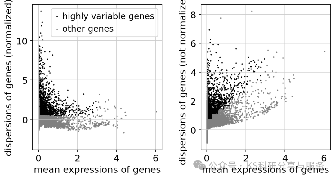

接下来是一个可选步骤，如果在计算完高变基因之后，你不再跑sc.pp.regress_out 进行数据校正，也不跑 sc.pp.scale 进行数据缩放，就没必要只保留高变基因用于后续的分析了。只保留高变基因用于后续分析只是为了降低数据维度，能够提高后续的分析效率，不跑adata = adata[:, adata.var.highly_variable]也是可以的，之前检测到的高变基因结果会作为注释存储在 .var.highly_variable 中，并且会被主成分分析（PCA）自动检测到，因此 sc.pp.neighbors 以及后续的manifold/graph工具也能自动检测到。

Cell-Cycle Scoring：在进行下一步之前，我觉得有必要插播一条内容，那就是细胞周期评分的计算，在seurat分析的时候，经常会用到了，有时候细胞周期可能影响后续的分析，需要回归掉，那么为了对接到seurat，scanpy这里也得介绍一下，虽然这个步骤并不是所有分析中都是必须的步骤。scanpy细胞周期评分思路与seurat一样。需要设定相关的基因。对于人的，scanpy提供了一个txt文件https://github.com/scverse/scanpy_usage/blob/master/180209_cell_cycle/data/regev_lab_cell_cycle_genes.txt。读取然后设置即可。对于其他物种，需要自行传入基因列表，其他步骤一样。

#读取周期基因，是一个list
cell_cycle_genes = [x.strip() for x in open('./regev_lab_cell_cycle_genes.txt')]
cell_cycle_genes[0:5]
#区分s_genes，g2m_genes，筛选出实际存在于当前数据集（adata）中的细胞周期基因
s_genes = cell_cycle_genes[:43]
g2m_genes = cell_cycle_genes[43:]
sc.tl.score_genes_cell_cycle(adata, s_genes=s_genes, g2m_genes=g2m_genes)
calculating cell cycle phase
computing score 'S_score'
WARNING: genes are not in var_names and ignored: Index(['MLF1IP'], dtype='object')
    finished: added
    'S_score', score of gene set (adata.obs).
    773 total control genes are used. (0:00:00)
computing score 'G2M_score'
WARNING: genes are not in var_names and ignored: Index(['FAM64A', 'HN1'], dtype='object')
    finished: added
    'G2M_score', score of gene set (adata.obs).
    729 total control genes are used. (0:00:00)
-->     'phase', cell cycle phase (adata.obs)
#可以看出，在我们演示的这个数据集下，细胞周期对于后续的分群没有显著的影响
sc.tl.pca(adata)
sc.pl.pca_scatter(adata, color='phase')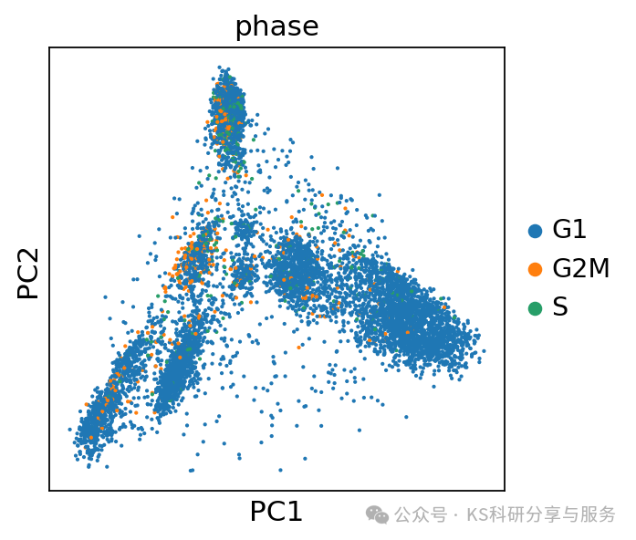

Regress out effects：这里其实也是可选步骤，如果协变量，例如测序深度、线粒体基因比例、核糖体基因比例、细胞周期等等会影响到后续的分析。那么可以选择将其回归掉这些影响。实际上，我们要视自己的数据来决定是否进行这些操作。使用sc.pp.regress_out进行回归，njobs参数可设置线程数。

sc.pp.regress_out(adata, ["total_counts", "pct_counts_mt"])
#数据缩放
sc.pp.scale(adata, max_value=10)
#暂时保存
adata.write_h5ad('./adata.h5ad')

后续将进行降维聚类，细胞注释分析！