文章目录
一、两层神经网络
下面是逻辑回归和两层神经网络的对比图:可以看出两层神经网络(激活函数为逻辑回归)就是做了两大次逻辑回归。
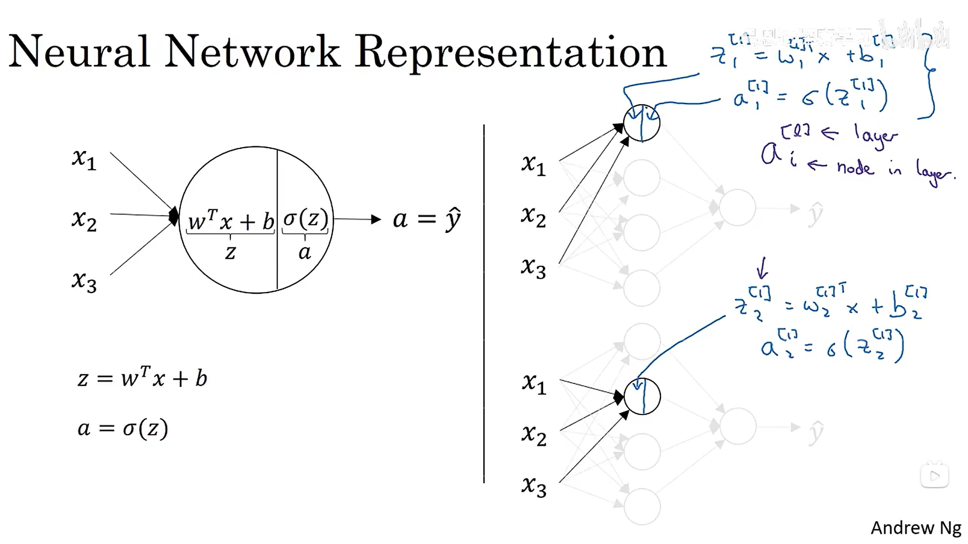
上述隐藏层的计算过程如下:每一个圈圈代表一个隐藏层单元,对应一个a值(做一次逻辑回归)。
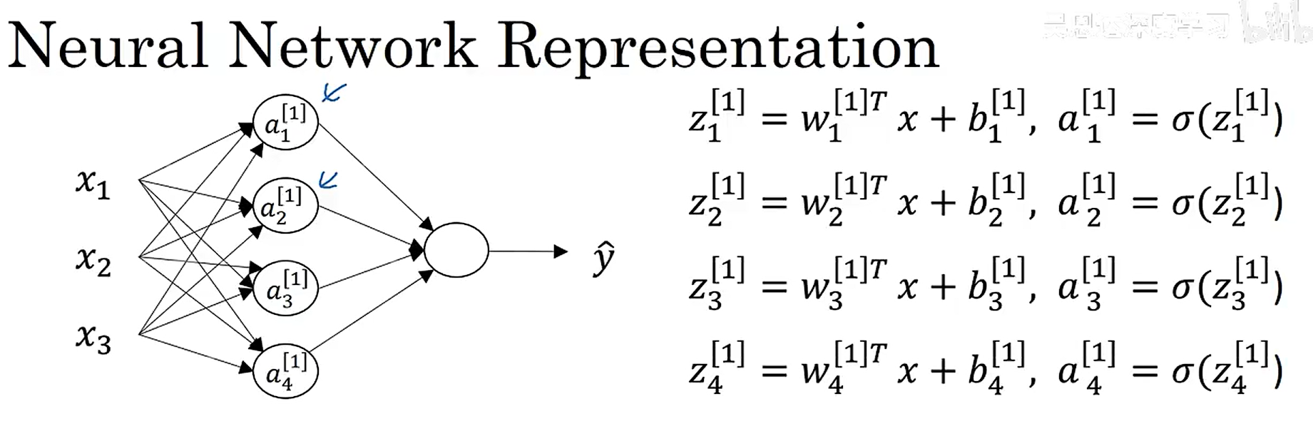
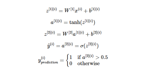
神经网络中两层的计算过程(矢量化计算)如下: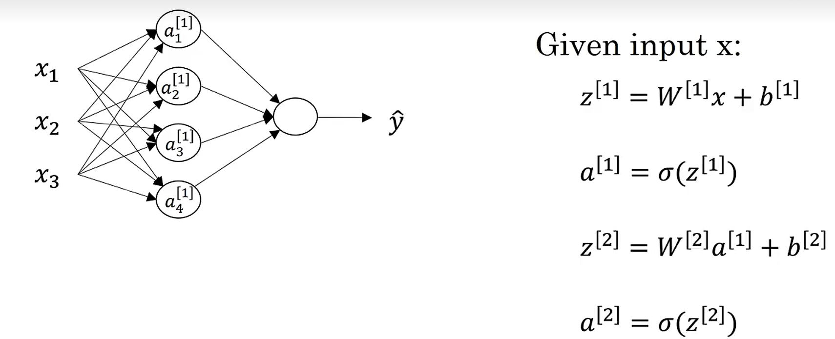
二、激活函数
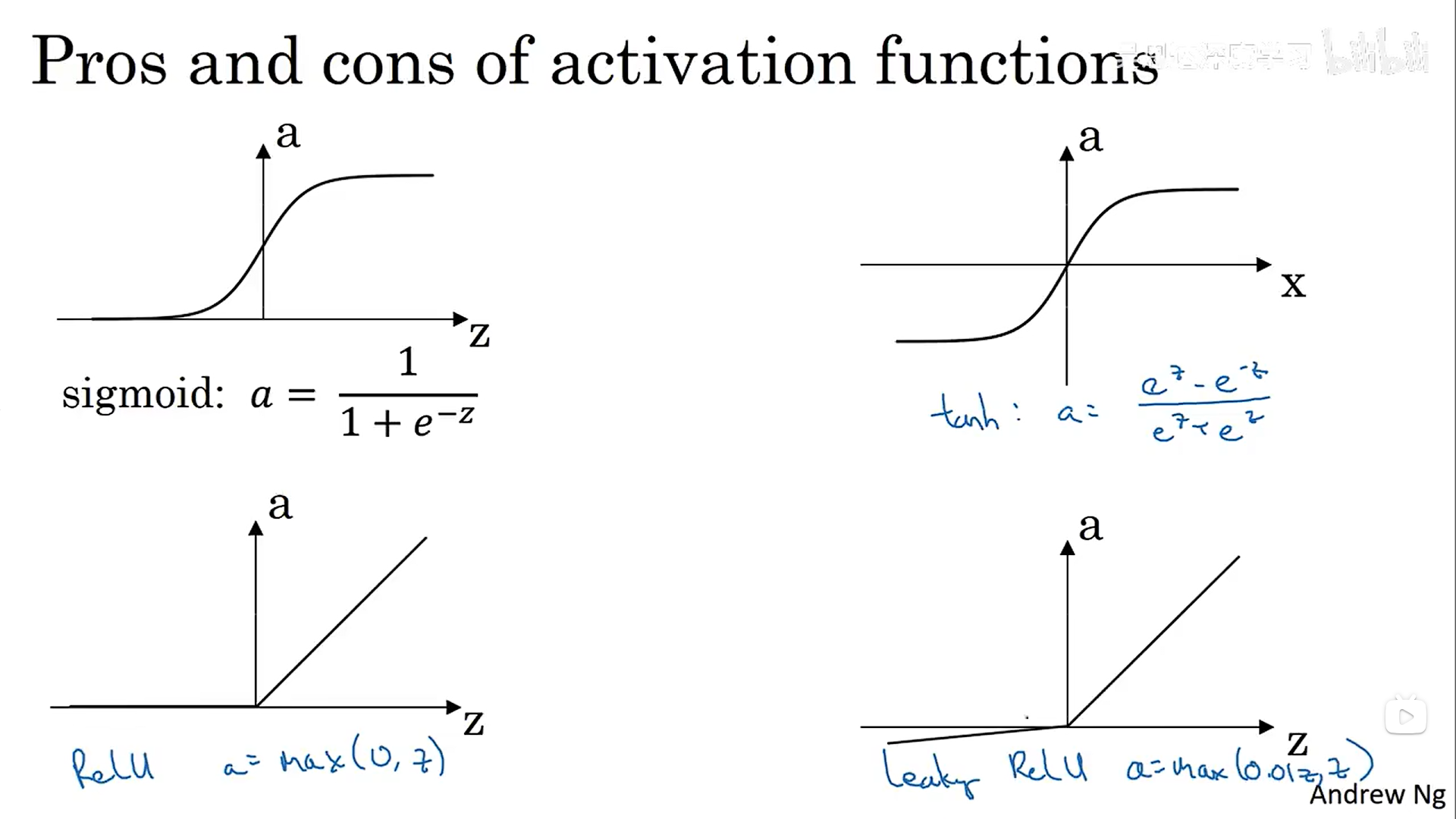
(一)激活函数的种类
这里提出了一种新的激活函数——tanh(),它是sigmois函数平移之后得到的,y坐标的值在-1和1之间。sigmoid函数和tanh函数有一个共同的缺点:在z无穷大时,函数的斜率接近0,会导致梯度下降变得非常缓慢,所以后面提出了relu激活函数(修正线性单元),现在作为默认的激活函数选择。relu没有当斜率为0时减慢梯度下降的效应。尽管函数当z为负数时,斜率为0,但是实际应用中,有足够多的隐藏单元令z大于0。
(二)神经网络为什么要使用非线性激活函数
在之前的机器学习课程中我们也提到过,如何使用线性激活函数,我们的神经网络输出结果跟直接使用线性回归没有什么区别。不管你的神经网络有多少层,最终做的只是计算线性激活函数。同样,如果你在所有隐藏层都使用线性回归,最终的输出层使用逻辑回归,这与你直接使用逻辑回归的结果是一样的。
(三)参数的初始化
当我们将所有的参数w和b全部初始化为0时,同一层的神经单元具有对称性,做的是相同的梯度下降,导致梯度下降过后的的各个神经单元的参数一模一样,导致多个隐藏单元没有意义。
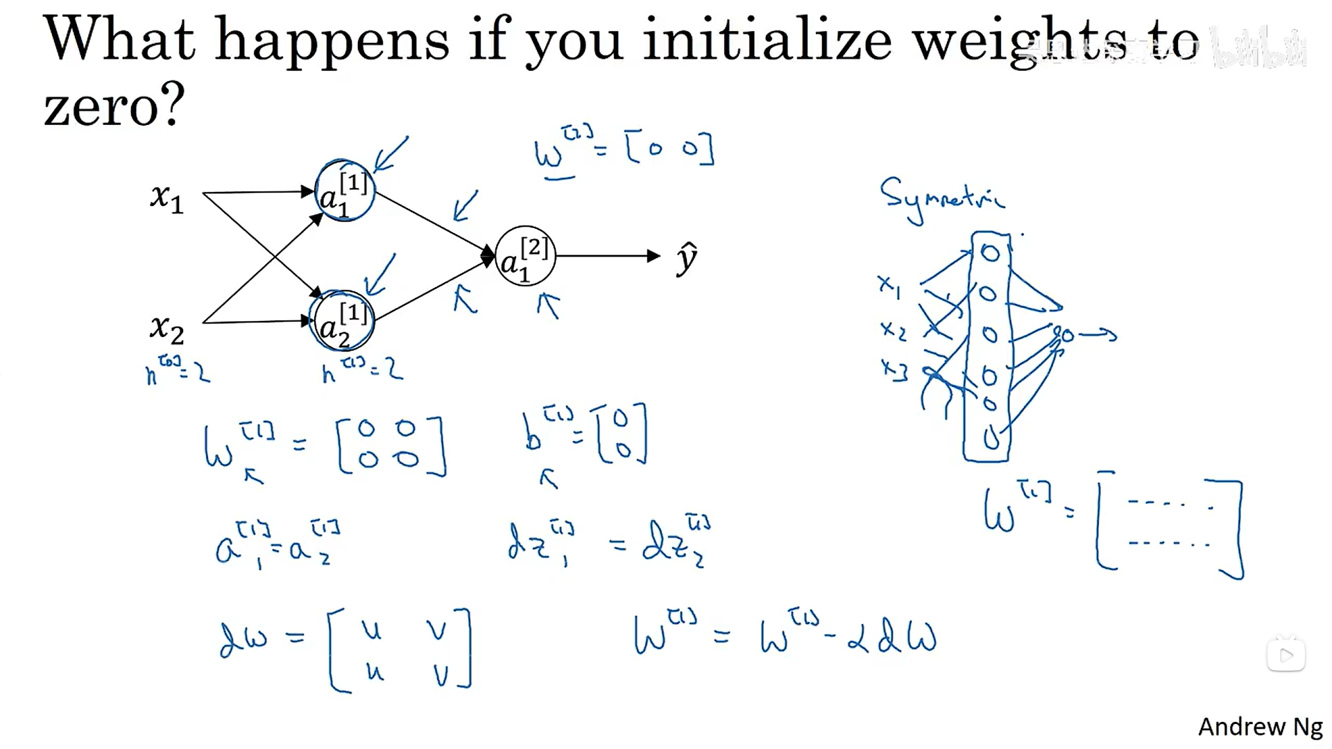
所以我们需要随机初始化参数:
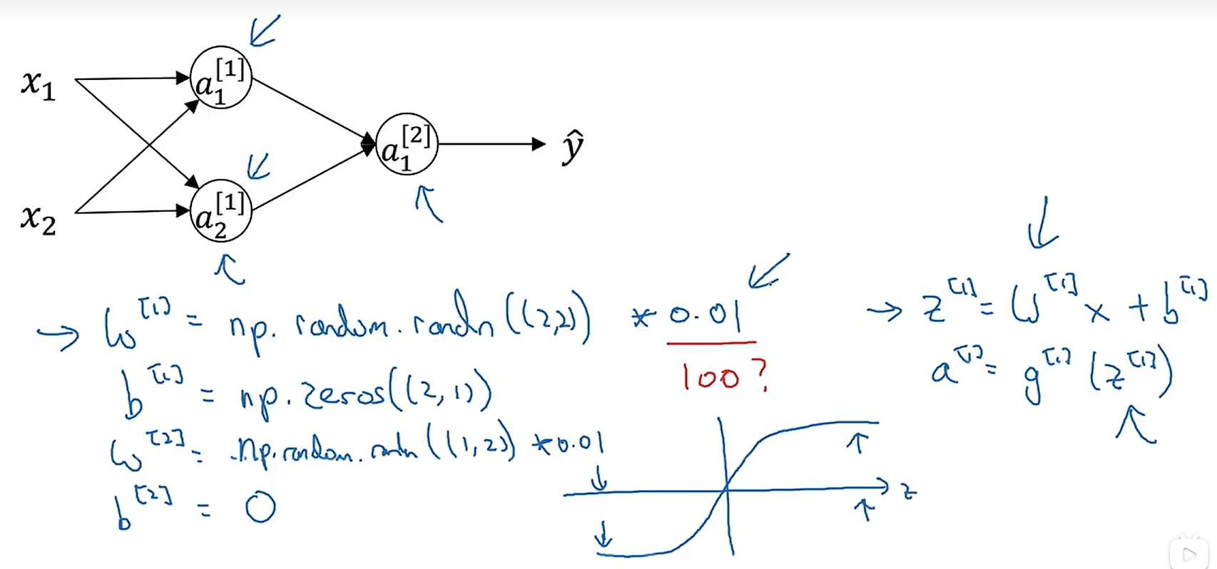
为什么生成符合正态分布的随机数之后还要×一个0.01,当我们的激活函数是sigmoid时,如果w太大,z就会越大,导致数据落在了激活函数较为平缓的区域,大大减慢了梯度下降的速度。0.01是一个比较合理的数值,当然如果不是sigmoid函数,我们也可以多多尝试一下其他的数值,后续会再讲这个数值的选择。
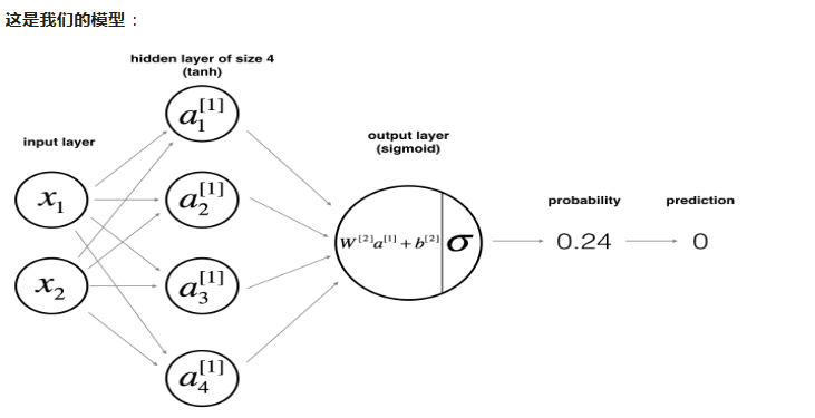
(四)构建具有一个隐藏层的分类神经网络
(1)数据集
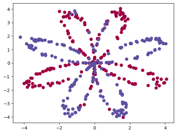
(2)使用逻辑回归直接拟合数据:准确率只有47%
# Train the logistic regression classifier
clf = sklearn.linear_model.LogisticRegressionCV();
clf.fit(X.T, Y[0, :].T);
(3)根据数据构建神经网络模型
Logistic 回归在“花卉数据集”上效果不佳。下面将训练具有单个隐藏层的神经网络。
计算成本的函数如下: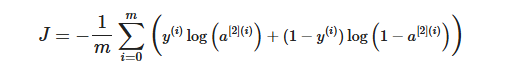
提醒: 构建神经网络的一般方法是:1. 定义神经网络结构(# 输入单元、# 隐藏单元等)。2. 初始化模型的参数 3.循环: - 实现前向传播 - 计算损失 - 实现向后传播以获得梯度 - 更新参数(梯度下降)。
(4)初始化模型的参数
# GRADED FUNCTION: initialize_parameters

def initialize_parameters(n_x, n_h, n_y):
    """
    Argument:
    n_x -- size of the input layer
    n_h -- size of the hidden layer
    n_y -- size of the output layer

    Returns:
    params -- python dictionary containing your parameters:
                    W1 -- weight matrix of shape (n_h, n_x)
                    b1 -- bias vector of shape (n_h, 1)
                    W2 -- weight matrix of shape (n_y, n_h)
                    b2 -- bias vector of shape (n_y, 1)
    """

    np.random.seed(2) # we set up a seed so that your output matches ours although the initialization is random.

    ### START CODE HERE ### (≈ 4 lines of code)
    W1 = np.random.randn(n_h,n_x)*0.01
    b1 = np.zeros((n_h,1))
    W2 = np.random.randn(n_y,n_h)*0.01
    b2 = np.zeros((n_y,1))
    ### END CODE HERE ###

    assert (W1.shape == (n_h, n_x))
    assert (b1.shape == (n_h, 1))
    assert (W2.shape == (n_y, n_h))
    assert (b2.shape == (n_y, 1))

    parameters = {"W1": W1,
                  "b1": b1,
                  "W2": W2,
                  "b2": b2}

    return parameters
(5)前向传播(矢量化)
# GRADED FUNCTION: forward_propagation

def forward_propagation(X, parameters):
    """
    Argument:
    X -- input data of size (n_x, m)
    parameters -- python dictionary containing your parameters (output of initialization function)

    Returns:
    A2 -- The sigmoid output of the second activation
    cache -- a dictionary containing "Z1", "A1", "Z2" and "A2"
    """
    # Retrieve each parameter from the dictionary "parameters"
    ### START CODE HERE ### (≈ 4 lines of code)
    W1 = parameters["W1"]
    b1 = parameters["b1"]
    W2 = parameters["W2"]
    b2 = parameters["b2"]
    ### END CODE HERE ###

    # Implement Forward Propagation to calculate A2 (probabilities)
    ### START CODE HERE ### (≈ 4 lines of code)
    Z1 = np.dot(W1,X)+b1
    A1 = np.tanh(Z1)
    Z2 = np.dot(W2,A1)+b2
    A2 = np.tanh(Z2)
    ### END CODE HERE ###

    assert(A2.shape == (1, X.shape[1]))

    cache = {"Z1": Z1,
             "A1": A1,
             "Z2": Z2,
             "A2": A2}

    return A2, cache
(6)计算成本函数

# GRADED FUNCTION: compute_cost

def compute_cost(A2, Y, parameters):
    """
    Computes the cross-entropy cost given in equation (13)

    Arguments:
    A2 -- The sigmoid output of the second activation, of shape (1, number of examples)
    Y -- "true" labels vector of shape (1, number of examples)
    parameters -- python dictionary containing your parameters W1, b1, W2 and b2

    Returns:
    cost -- cross-entropy cost given equation (13)
    """

    m = Y.shape[1] # number of example

    # Compute the cross-entropy cost
    ### START CODE HERE ### (≈ 2 lines of code)
    logprobs = np.multiply(np.log(A2),Y)+np.multiply(np.log(1-A2),1-Y)
    cost = np.sum(logprobs)/-m
                    # no need to use a for loop!

    ### END CODE HERE ###

    cost = np.squeeze(cost)     # makes sure cost is the dimension we expect.
                                # E.g., turns [[17]] into 17
    assert(isinstance(cost, float))

    return cost
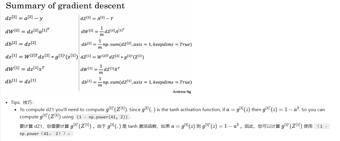
(7)根据导数计算公式进行向后传播
# GRADED FUNCTION: backward_propagation

def backward_propagation(parameters, cache, X, Y):
    """
    Implement the backward propagation using the instructions above.

    Arguments:
    parameters -- python dictionary containing our parameters
    cache -- a dictionary containing "Z1", "A1", "Z2" and "A2".
    X -- input data of shape (2, number of examples)
    Y -- "true" labels vector of shape (1, number of examples)

    Returns:
    grads -- python dictionary containing your gradients with respect to different parameters
    """
    m = X.shape[1]

    # First, retrieve W1 and W2 from the dictionary "parameters".
    ### START CODE HERE ### (≈ 2 lines of code)
    W1 = parameters["W1"]
    W2 = parameters["W2"]
    print(W1.shape)
    print(W2.shape)
    ### END CODE HERE ###

    # Retrieve also A1 and A2 from dictionary "cache".
    ### START CODE HERE ### (≈ 2 lines of code)
    A1 = cache["A1"]
    A2 = cache["A2"]
    print(A1.shape)
    print(A2.shape)
    ### END CODE HERE ###

    # Backward propagation: calculate dW1, db1, dW2, db2.
    ### START CODE HERE ### (≈ 6 lines of code, corresponding to 6 equations on slide above)
    dZ2 = A2-Y
    dW2 = np.dot(dZ2,A1.T)/m
    db2 = np.sum(dZ2,axis = 1,keepdims=True)/m
    dZ1 = np.dot(W2.T,dZ2)*(1-np.power(A1,2))
    dW1 = np.dot(dZ1,X.T)/m
    db1 = np.sum(dZ1,axis = 1,keepdims=True)/m
    ### END CODE HERE ###

    grads = {"dW1": dW1,
             "db1": db1,
             "dW2": dW2,
             "db2": db2}

    return grads
其中的cache是在进行向前传播时,将计算过程中关于A1和A2的变量缓存保存了下来,提供给计算梯度使用。
# GRADED FUNCTION: update_parameters

def update_parameters(parameters, grads, learning_rate = 1.2):
    """
    Updates parameters using the gradient descent update rule given above

    Arguments:
    parameters -- python dictionary containing your parameters
    grads -- python dictionary containing your gradients

    Returns:
    parameters -- python dictionary containing your updated parameters
    """
    # Retrieve each parameter from the dictionary "parameters"
    ### START CODE HERE ### (≈ 4 lines of code)
    W1 = parameters["W1"]
    b1 = parameters["b1"]
    W2 = parameters["W2"]
    b2 = parameters["b2"]
    ### END CODE HERE ###

    # Retrieve each gradient from the dictionary "grads"
    ### START CODE HERE ### (≈ 4 lines of code)
    dW1 = grads["dW1"]
    db1 = grads["db1"]
    dW2 = grads["dW2"]
    db2 = grads["db2"]
    ## END CODE HERE ###

    # Update rule for each parameter
    ### START CODE HERE ### (≈ 4 lines of code)
    W1 = W1 - dW1*learning_rate
    b1 = b1 - db1*learning_rate
    W2 = W2 - dW2*learning_rate
    b2 = b2 - db2*learning_rate

    ### END CODE HERE ###

    parameters = {"W1": W1,
                  "b1": b1,
                  "W2": W2,
                  "b2": b2}

    return parameters
(8)集成上述辅助函数
# GRADED FUNCTION: nn_model

def nn_model(X, Y, n_h, num_iterations = 10000, print_cost=False):
    """
    Arguments:
    X -- dataset of shape (2, number of examples)
    Y -- labels of shape (1, number of examples)
    n_h -- size of the hidden layer
    num_iterations -- Number of iterations in gradient descent loop
    print_cost -- if True, print the cost every 1000 iterations

    Returns:
    parameters -- parameters learnt by the model. They can then be used to predict.
    """

    np.random.seed(3)
    n_x = layer_sizes(X, Y)[0]
    n_y = layer_sizes(X, Y)[2]

    # Initialize parameters, then retrieve W1, b1, W2, b2. Inputs: "n_x, n_h, n_y". Outputs = "W1, b1, W2, b2, parameters".
    ### START CODE HERE ### (≈ 5 lines of code)
    parameters = initialize_parameters(n_x, n_h, n_y)
    W1 = parameters["W1"]
    b1 = parameters["b1"]
    W2 = parameters["W2"]
    b2 = parameters["b2"]
    ### END CODE HERE ###

    # Loop (gradient descent)

    for i in range(0, num_iterations):

        ### START CODE HERE ### (≈ 4 lines of code)
        # Forward propagation. Inputs: "X, parameters". Outputs: "A2, cache".
        A2,cache = forward_propagation(X, parameters)
        # Cost function. Inputs: "A2, Y, parameters". Outputs: "cost".
        cost = compute_cost(A2, Y, parameters)
        # Backpropagation. Inputs: "parameters, cache, X, Y". Outputs: "grads".
        grads = backward_propagation(parameters, cache, X, Y)
        # Gradient descent parameter update. Inputs: "parameters, grads". Outputs: "parameters".
        parameters = update_parameters(parameters, grads, learning_rate = 1.2)
        ### END CODE HERE ###

        # Print the cost every 1000 iterations
        if print_cost and i % 1000 == 0:
            print ("Cost after iteration %i: %f" %(i, cost))

    return parameters
(9)使用模型进行预测
# GRADED FUNCTION: predict

def predict(parameters, X):
    """
    Using the learned parameters, predicts a class for each example in X

    Arguments:
    parameters -- python dictionary containing your parameters
    X -- input data of size (n_x, m)

    Returns
    predictions -- vector of predictions of our model (red: 0 / blue: 1)
    """

    # Computes probabilities using forward propagation, and classifies to 0/1 using 0.5 as the threshold.
    ### START CODE HERE ### (≈ 2 lines of code)
    W1 = parameters["W1"]
    b1 = parameters["b1"]
    W2 = parameters["W2"]
    b2 = parameters["b2"]
    Z1 = np.dot(W1,X)+b1
    A1 = np.tanh(Z1)
    Z2 = np.dot(W2,A1)+b2
    predictions = np.tanh(Z2)

    ### END CODE HERE ###

    return predictions
使用神经网络模型进行训练,准确率达到90%。同时我们可以设置不同的隐藏层中的隐藏单元个数,看看模型的准确率的变化情况,从而选择最佳的隐藏单元个数。