一、前言
最近在做导航相关的项目,所以顺便来学习一下相关的导航相关的定位原理,顺便写一写自己的理解,以及记录相关数学知识。
二、交会定位方法
在一个二维平面中,规定坐标方位角,如下图:
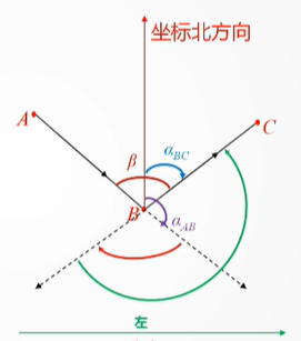
规定坐标北方向,为方位角基准,角度计算是以顺时针旋转为基准,即满足下面的公式:
当β为左角时:
当β为右角时:
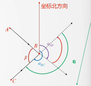
满足如下公式:
已知上面的坐标角度的定义了,来看一个例子,加上三角函数的知识,求出下图P点的坐标。
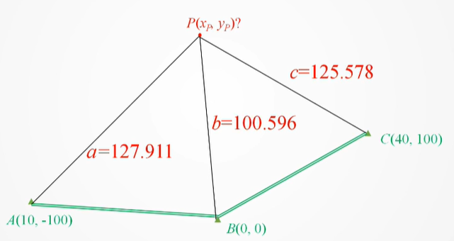
在三角形ABP中,基于上面所讲的坐标正正北方向,满足如下条件:
代码实现如下:
    float a=127.911,b=100.596,A_x=-100.0,A_y=10.0,B_x=0.0,B_y=0.0,P_x,P_y;
    float cosA,atanA_1,deg_AP;
    float L_ab= sqrt(pow(A_x-B_x,2)+pow(A_y-B_y,2));
    cosA=(pow(L_ab,2)+pow(a,2)-pow(b,2))/(2*a*L_ab);
    atanA_1=atan((A_y-B_y)/(B_x-A_x));  //这个计算的是AB反正切求弧度,为了求出AP与正北的夹角
    deg_AP = atanA_1*180.0/3.1415926+90.0-acos(cosA)*180.0/3.1415926;

    P_x = A_x + a*sin(deg_AP * 3.1415926 / 180.0);
    P_y = A_y + a*cos(deg_AP * 3.1415926 / 180.0);
三、三点距离交会法
如下图所示,三点交会的示意图:
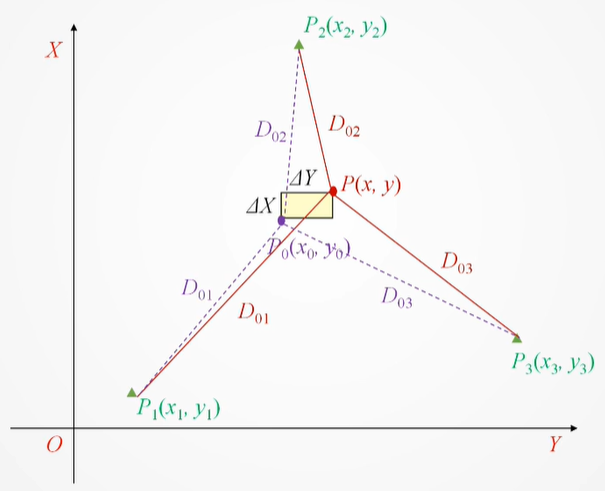
从上线的几何关系可以得出,如下的三个非线性方程:
直接从这个方程组求解(x,y)非常困难。我们需要一种方法把它变成我们熟悉的,容易求解的线性方程组(如 ax + by =c)。
3.1.线性化的核心策略 ——泰勒展开
核心思想:任何一个光滑函数,都可以在一个已知的、非常接近真实值的“近似点”附近,用一条直线(或一个平面)来非常精确得近似它。
在我们的问题中:
1.我们不知道真实的点 P 的坐标 (X, Y)。
2.但我们先猜一个(或通过简单计算得到一个)近似坐标 P₀(X₀, Y₀)。这个点应该离真实点 P 不远。
3.真实的坐标 (X, Y) 就等于近似坐标加上一个很小的修正量 (ΔX, ΔY):
4.我们的目标从求解 (X, Y) 转变为求解很小的修正量 (ΔX, ΔY)。
我们关注其中一个方程,函数是距离函数:
这个函数代表了从点 P 到已知点 P_i 的真实距离。
执行泰勒展开(最关键的一步)
我们现在要把函数 f(X, Y) 在近似点 (X₀, Y₀) 处进行一阶泰勒展开。
我们先来看看泰勒展开的基本公式如下:
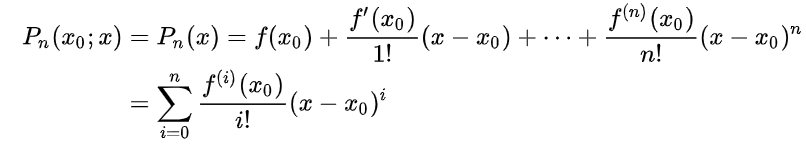
我们是一阶线性展开,对于任何函数f(x,y),在点(x0,y0)附近的展开式为:
令:
我们记 a_i = (X₀ - X_i) / d_i。这个 a_i 其实就是从P_i指向P₀的方向向量的X分量(单位向量),然后将X=X0 + ΔX 带入之前的距离公式,可以的到如下式子:
把上面的式子移项整理,把所有已知量放在右边,未知量 (v_i, ΔX, ΔY) 放在左边:
v_i:观测值的改正数(也是未知数,但后续可用最小二乘法处理)(d_i - D_i):常数项。它是“根据近似坐标计算的距离”减去“实际观测的距离”,也称为闭合差。如果我们的近似坐标很好且观测没有误差,这个值应该接近0。a_i,b_i:系数。是已知的、从几何关系中计算出来的方向余弦。ΔX,ΔY:待求的未知数。是我们需要求解的坐标修正量。
3.2.最小二乘法
根据上面的推导,我们可可以得到三个线性化的误差方程:
将上述方程组写成矩阵形式:
其中:
是改正数向量
是常数项向量
是系数矩阵
最小二乘准则
最小二乘准则要求改正数的平方和最小:
代入矩阵表达式:
求解极小值
对φ求关于X的偏导数并令其为零:
最小二乘法的接法方程如下:
解法方程得到未知数向量的解,整理得:
更新坐标
得到δx 和δy后,更新坐标:
我们需要先选取一个初始近似点P0。初始近似点可以选择三个已知点的重心,或者通过其他方法估计。
四、代码实现
以上就是三点交会定位的方法推导流程,接下来就是附上代码示例:
#include <stdio.h>
#include <math.h>
#include <stdlib.h>

// 定义点结构体
typedef struct {
    double x;
    double y;
} Point;

// 定义已知点和观测距离
typedef struct {
    Point point;
    double distance;
} KnownPoint;

// 计算两点之间的距离
double calculate_distance(Point p1, Point p2) {
    return sqrt(pow(p1.x - p2.x, 2) + pow(p1.y - p2.y, 2));
}

/**
 * @brief 最小二乘解算函数
 */
Point least_squares_solution(Point initial_guess, KnownPoint points[], int num_points, double tolerance, int max_iterations) {
    Point current = initial_guess;
    int iteration = 0;
    double delta_x, delta_y;

    do {
        // 构建矩阵A和向量L
        double *a = malloc(num_points * sizeof(double));
        double *b = malloc(num_points * sizeof(double));
        double *l = malloc(num_points * sizeof(double));

        //A^T * A 的计算
        for (int i = 0; i < num_points; i++) {
            double d = calculate_distance(current, points[i].point);
            a[i] = (current.x - points[i].point.x) / d;
            b[i] = (current.y - points[i].point.y) / d;
            l[i] = d - points[i].distance;
        }

        // 计算法方程系数
        double ata11 = 0, ata12 = 0, ata22 = 0;
        double atl1 = 0, atl2 = 0;

         //A^T * L 的计算
        for (int i = 0; i < num_points; i++) {
            ata11 += a[i] * a[i];
            ata12 += a[i] * b[i];
            ata22 += b[i] * b[i];

            atl1 += a[i] * l[i];
            atl2 += b[i] * l[i];
        }

        // 小规模矩阵,使用克莱姆法则解法方程
        double determinant = ata11 * ata22 - ata12 * ata12;
        if (fabs(determinant) < 1e-10) {
            printf("警告:法方程矩阵接近奇异,解可能不可靠。\n");
        }

        delta_x = (ata22 * (-atl1) - ata12 * (-atl2)) / determinant;
        delta_y = (ata11 * (-atl2) - ata12 * (-atl1)) / determinant;

        // 更新坐标
        current.x += delta_x;
        current.y += delta_y;

        // 释放内存
        free(a);
        free(b);
        free(l);

        iteration++;

        // 打印迭代信息
        printf("迭代 %d: ΔX = %.6f, ΔY = %.6f, 新坐标: (%.6f, %.6f)\n",
               iteration, delta_x, delta_y, current.x, current.y);

    } while ((fabs(delta_x) > tolerance || fabs(delta_y) > tolerance) && iteration < max_iterations);

    if (iteration >= max_iterations) {
        printf("达到最大迭代次数,可能未收敛。\n");
    } else {
        printf("收敛于 %d 次迭代。\n", iteration);
    }

    return current;
}

int main() {
    // 设置已知点和观测距离
    KnownPoint points[3];
    points[0].point.x = 10; points[0].point.y = -100; points[0].distance = 127.911;
    points[1].point.x = 0;  points[1].point.y = 0;    points[1].distance = 100.596;
    points[2].point.x = 40; points[2].point.y = 100;  points[2].distance = 125.578;

    // 初始猜测坐标
    Point initial_guess = {50.0, 0.0}; // 可以设置为已知点的重心或其他合理估计

    // 解算参数
    double tolerance = 1e-6; // 收敛容差
    int max_iterations = 100; // 最大迭代次数

    printf("三点距离交会法最小二乘解算\n");
    printf("已知点:\n");
    printf("A(%.3f, %.3f), D1 = %.3f\n", points[0].point.x, points[0].point.y, points[0].distance);
    printf("B(%.3f, %.3f), D2 = %.3f\n", points[1].point.x, points[1].point.y, points[1].distance);
    printf("C(%.3f, %.3f), D3 = %.3f\n", points[2].point.x, points[2].point.y, points[2].distance);
    printf("初始近似坐标: (%.3f, %.3f)\n", initial_guess.x, initial_guess.y);
    printf("收敛容差: %.6f\n", tolerance);
    printf("最大迭代次数: %d\n\n", max_iterations);

    // 执行解算
    Point solution = least_squares_solution(initial_guess, points, 3, tolerance, max_iterations);

    // 输出最终结果
    printf("\n最终解算结果:\n");
    printf("P点坐标: (%.6f, %.6f)\n", solution.x, solution.y);

    // 计算残差
    printf("\n残差分析:\n");
    for (int i = 0; i < 3; i++) {
        double calculated_distance = calculate_distance(solution, points[i].point);
        double residual = calculated_distance - points[i].distance;
        printf("到点%d: 观测距离 = %.6f, 计算距离 = %.6f, 残差 = %.6f\n",
               i+1, points[i].distance, calculated_distance, residual);
    }

    return 0;
}
代码运行结果:
三点距离交会法最小二乘解算
已知点:
A(10.000, -100.000), D1 = 127.911
B(0.000, 0.000), D2 = 100.596
C(40.000, 100.000), D3 = 125.578
初始近似坐标: (50.000, 0.000)
收敛容差: 0.000001
最大迭代次数: 100迭代 1: ΔX = 55.073416, ΔY = -10.652607, 新坐标: (105.073416, -10.652607)
迭代 2: ΔX = -4.633618, ΔY = 0.804377, 新坐标: (100.439798, -9.848230)
迭代 3: ΔX = -0.044214, ΔY = 0.004803, 新坐标: (100.395584, -9.843427)
迭代 4: ΔX = -0.000063, ΔY = 0.000011, 新坐标: (100.395521, -9.843416)
迭代 5: ΔX = -0.000000, ΔY = 0.000000, 新坐标: (100.395521, -9.843416)
收敛于 5 次迭代。最终解算结果:
P点坐标: (100.395521, -9.843416)残差分析:
到点1: 观测距离 = 127.911000, 计算距离 = 127.669729, 残差 = -0.241271
到点2: 观测距离 = 100.596000, 计算距离 = 100.876922, 残差 = 0.280922
到点3: 观测距离 = 125.578000, 计算距离 = 125.352284, 残差 = -0.225716
思考:
二维平面可以通过这样的方式进行定位计算,那么三位是不是也可以这样做呢?
卫星定位原理:
1颗卫星:你知道你在一个以卫星为球心、以伪距为半径的大球面上的某处。位置无法确定。
2颗卫星:两个大球面相交,会得到一个圆圈。你在这个圆圈上的某点。
3颗卫星:三个球面相交,通常会得到两个点。其中一个点在地球上,另一个点可能在太空中。通过算法排除掉不合理的点,理论上可以确定你的地面位置(经度、纬度、高度)。但是,如果接收器时钟不准,3颗卫星的解算误差会非常大。
4颗卫星:四个球面相交,唯一确定一个点。这个点就是你的准确位置,并且还能精确校准你的接收器时钟。