
简 介
Cox比例风险回归模型已成为医学研究中生存数据建模的传统选择。为了在Cox模型中引入灵活性,可以应用几种平滑方法,在这种情况下,基于样条的方法是最常考虑的。为了更好地理解每个连续协变量对结果的影响,结果可以用基于样条的风险比(HR)曲线表示,以特定的协变量值为参考。尽管在生存分析中使用样条平滑方法具有潜在的优势,但目前在R软件中没有分析方法来选择多变量Cox模型(具有两个或多个非线性协变量效应)的最佳自由度。本文描述了一个R包,称为smoothHR,允许计算非线性引入的连续预测器的HR的逐点估计及其相应的置信限。此外,该软件包还提供了在多变量Cox模型中自动选择自由度的功能。使用急性冠状动脉综合征数据来说明smoothHR包的关键功能的使用。
软件安装
if(!require(smoothHR))
  install.packages("smoothHR")
library(smoothHR)
library(survival)函数说明
Function |
Description |
|---|---|
smoothHR |
Main function of the package. Returns an object of class HR. |
dfmacox |
Provides the number of degrees of freedom in the additive Cox model. |
plot |
A function that provides the plots for the hazard ratio curves taking a specific value as reference. |
predict |
Provides estimates for the hazard ratio and their corresponding confidence limits. |
Prints details about the Cox model. |
实例操作
数据读取
data("whas500")
head(whas500)
## id age gender hr sysbp diasbp bmi cvd afb sho chf av3 miord mitype year
## 1 1 83 0 89 152 78 25.54051 1 1 0 0 0 1 0 1
## 2 2 49 0 84 120 60 24.02398 1 0 0 0 0 0 1 1
## 3 3 70 1 83 147 88 22.14290 0 0 0 0 0 0 1 1
## 4 4 70 0 65 123 76 26.63187 1 0 0 1 0 0 1 1
## 5 5 70 0 63 135 85 24.41255 1 0 0 0 0 0 1 1
## 6 6 70 0 76 83 54 23.24236 1 0 0 0 1 0 0 1
## admitdate disdate fdate los dstat lenfol fstat
## 1 13-01-1997 18-01-1997 31-12-2002 5 0 2178 0
## 2 19-01-1997 24-01-1997 31-12-2002 5 0 2172 0
## 3 01-01-1997 06-01-1997 31-12-2002 5 0 2190 0
## 4 17-02-1997 27-02-1997 11-12-1997 10 0 297 1
## 5 01-03-1997 07-03-1997 31-12-2002 6 0 2131 0
## 6 11-03-1997 12-03-1997 12-03-1997 1 1 1 1whas500=whas500[,-c(1,16,17,18)]单变量
预测变量 bmi
smoothHR函数提供灵活的危险比曲线,允许连续预测变量与生存之间的非线性关系。为了更好地理解每个连续协变量对结果的影响,结果以危险比曲线的形式表示,以特定协变量值为参考。这些曲线的置信区间也已推导出来。
smoother:使用‘ns’表示自然样条平滑或使用‘pspline’表示惩罚样条平滑。
fit <- coxph(Surv(lenfol, fstat)~age+hr+gender+diasbp+pspline(bmi)+pspline(los),
             data=whas500, x=TRUE)
hr1 <- smoothHR(data=whas500, coxfit=fit)
hr1
##
## Cox Proportional Hazards Model
## Call:
## coxph(formula = Surv(lenfol, fstat) ~ age + hr + gender + diasbp +
## pspline(bmi) + pspline(los), data = whas500, x = TRUE)
##
## coef se(coef) se2 Chisq DF p
## age 0.05682 0.00668 0.00667 72.37950 1.00 < 2e-16
## hr 0.01391 0.00284 0.00283 23.94579 1.00 9.9e-07
## gender -0.25071 0.14393 0.14362 3.03404 1.00 0.08154
## diasbp -0.01188 0.00359 0.00357 10.96060 1.00 0.00093
## pspline(bmi), linear -0.03725 0.01438 0.01435 6.70986 1.00 0.00959
## pspline(bmi), nonlin 10.48506 3.08 0.01598
## pspline(los), linear 0.01310 0.01479 0.01465 0.78371 1.00 0.37601
## pspline(los), nonlin 10.70873 2.95 0.01280
##
## Iterations: 4 outer, 15 Newton-Raphson
## Theta= 0.799
## Theta= 0.366
## Degrees of freedom for terms= 1.0 1.0 1.0 1.0 4.1 3.9
## Likelihood ratio test=202 on 12 df, p=<2e-16
## n= 500, number of events= 215
##
## Proportional Hazards Assumption
## chisq df p
## age 0.151 1.00 0.70
## hr 1.680 0.99 0.19
## gender 0.114 1.00 0.73
## diasbp 1.702 0.99 0.19
## pspline(bmi) 1.147 4.08 0.89
## pspline(los) 3.625 3.95 0.45
## GLOBAL 8.664 12.01 0.73predict(hr1, predictor="bmi",prob=0, conf.level=0.95)## bmi LnHR lower .95 upper .95
## 13.04546 1.26624009 0.1015945 2.4308856
## 18.60004 0.79522426 0.2601568 1.3302917
## 23.22377 0.32722547 -0.1670588 0.8215097
## 25.94593 0.15487865 -0.3343962 0.6441535
## 29.39196 0.08437564 -0.3271063 0.4958576
## 36.77345 0.10139527 -0.2230930 0.4258835
## 44.83886 1.63447099 -0.1676770 3.4366190plot(hr1, predictor="bmi", prob=0, conf.level=0.95)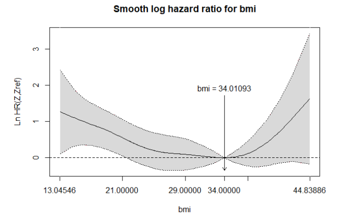
预测变量 los
# Example 2
hr2 <- smoothHR(data=whas500, time="lenfol", status="fstat", formula=~age+hr+gender+diasbp+
                   pspline(bmi)+pspline(los) )
hr2
##
## Cox Proportional Hazards Model
## Call:
## coxph(formula = covar2, data = data, x = TRUE)
##
## coef se(coef) se2 Chisq DF p
## age 0.05682 0.00668 0.00667 72.37950 1.00 < 2e-16
## hr 0.01391 0.00284 0.00283 23.94579 1.00 9.9e-07
## gender -0.25071 0.14393 0.14362 3.03404 1.00 0.08154
## diasbp -0.01188 0.00359 0.00357 10.96060 1.00 0.00093
## pspline(bmi), linear -0.03725 0.01438 0.01435 6.70986 1.00 0.00959
## pspline(bmi), nonlin 10.48506 3.08 0.01598
## pspline(los), linear 0.01310 0.01479 0.01465 0.78371 1.00 0.37601
## pspline(los), nonlin 10.70873 2.95 0.01280
##
## Iterations: 4 outer, 15 Newton-Raphson
## Theta= 0.799
## Theta= 0.366
## Degrees of freedom for terms= 1.0 1.0 1.0 1.0 4.1 3.9
## Likelihood ratio test=202 on 12 df, p=<2e-16
## n= 500, number of events= 215
##
## Proportional Hazards Assumption
## chisq df p
## age 0.151 1.00 0.70
## hr 1.680 0.99 0.19
## gender 0.114 1.00 0.73
## diasbp 1.702 0.99 0.19
## pspline(bmi) 1.147 4.08 0.89
## pspline(los) 3.625 3.95 0.45
## GLOBAL 8.664 12.01 0.73plot(hr2, predictor="los", pred.value=7, conf.level=0.95, xlim=c(0,30), round.x=1,
ref.label="Ref.", xaxt="n")
xx <- c(0, 5, 10, 15, 20, 25, 30)
axis(1, xx)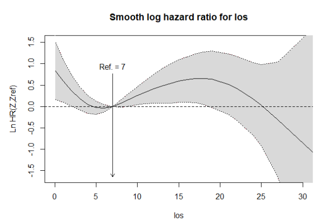
多变量预测
最佳自由度
dfmacox函数提供多元加性Cox模型中连续变量的自由度。
smoother:使用‘ns’表示自然样条平滑或使用‘pspline’表示惩罚样条平滑。
df<-dfmacox (time= "lenfol",
              status = "fstat",
              nl.predictors = c("los","bmi"),
              smoother = "ns",
              method = "AIC",
              data = whas500)

df
## $df
## [1] 5 3
##
## $AIC
## [1] 2402.863
##
## $AICc
## [1] 2405.741
##
## $BIC
## [1] 2429.828
##
## $myfit
## Call:
## coxph(formula = covar, data = data, x = TRUE)
##
## coef exp(coef) se(coef) z p
## ns(los, df = 5)1 -1.08402 0.33823 0.50353 -2.153 0.031329
## ns(los, df = 5)2 -0.67123 0.51108 0.58116 -1.155 0.248095
## ns(los, df = 5)3 0.35597 1.42757 0.76262 0.467 0.640660
## ns(los, df = 5)4 -1.64547 0.19292 1.62033 -1.016 0.309863
## ns(los, df = 5)5 -2.79503 0.06111 2.46344 -1.135 0.256543
## ns(bmi, df = 3)1 -2.12495 0.11944 0.35038 -6.065 1.32e-09
## ns(bmi, df = 3)2 -3.42648 0.03250 0.93599 -3.661 0.000251
## ns(bmi, df = 3)3 -1.41460 0.24302 0.67465 -2.097 0.036011
##
## Likelihood ratio test=67.78 on 8 df, p=1.359e-11
## n= 500, number of events= 215
##
## $method
## [1] "AIC"
##
## $nl.predictors
## [1] "los" "bmi"模型
hr<-smoothHR (time = "lenfol",
               status = "fstat",
               formula = ~ age+hr+gender+diasbp+ns(los,df = df$df[1]) + ns(bmi,df = df$df[2]),
               data = whas500)
## Warning: a global p-value of 0.003231001 was obtained when testing the proportional hazards assumptionhr##
## Cox Proportional Hazards Model
## Call:
## coxph(formula = covar2, data = data, x = TRUE)
##
## coef exp(coef) se(coef) z p
## age 0.056909 1.058559 0.006649 8.559 < 2e-16
## hr 0.013137 1.013224 0.002851 4.608 4.06e-06
## gender -0.281880 0.754364 0.145342 -1.939 0.052449
## diasbp -0.012158 0.987916 0.003594 -3.383 0.000717
## ns(los, df = df$df[1])1 -1.343838 0.260843 0.472188 -2.846 0.004427
## ns(los, df = df$df[1])2 -0.945611 0.388442 0.528033 -1.791 0.073323
## ns(los, df = df$df[1])3 0.495734 1.641704 0.820685 0.604 0.545810
## ns(los, df = df$df[1])4 -2.192518 0.111635 1.575252 -1.392 0.163967
## ns(los, df = df$df[1])5 -3.468907 0.031151 2.682442 -1.293 0.195945
## ns(bmi, df = df$df[2])1 -1.245960 0.287665 0.367896 -3.387 0.000707
## ns(bmi, df = df$df[2])2 -1.736646 0.176110 0.963655 -1.802 0.071522
## ns(bmi, df = df$df[2])3 0.068811 1.071234 0.708477 0.097 0.922627
##
## Likelihood ratio test=202.2 on 12 df, p=< 2.2e-16
## n= 500, number of events= 215
##
## Proportional Hazards Assumption
## chisq df p
## age 0.0965 1 0.75612
## hr 1.4437 1 0.22954
## gender 0.1176 1 0.73166
## diasbp 1.6065 1 0.20499
## ns(los, df = df$df[1]) 20.8522 5 0.00086
## ns(bmi, df = df$df[2]) 1.1194 3 0.77240
## GLOBAL 29.5779 12 0.00323预测 bmi
predict(hr, predictor="bmi",prob=0, conf.level=0.95)## bmi LnHR lower .95 upper .95
## 13.04546 1.326051223 0.55052797 2.10157448
## 18.60004 0.759738404 0.33283311 1.18664369
## 23.22377 0.345034967 -0.04459653 0.73466646
## 25.94593 0.146728035 -0.10057624 0.39403231
## 29.39196 0.007701568 -0.03469179 0.05009492
## 36.77345 0.235040407 -0.19489517 0.66497599
## 44.83886 0.948868529 -0.51493298 2.41267004plot(hr, predictor="bmi", prob=0, conf.level=0.95)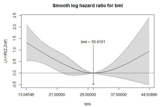
预测 los
predict(hr, predictor="los",prob=0, conf.level=0.95)## los LnHR lower .95 upper .95
## 0 3.681116 -1.686905 9.049137
## 1 3.476634 -1.791917 8.745185
## 3 2.842280 -2.424873 8.109432
## 5 2.528928 -2.682302 7.740159
## 7 2.803987 -2.363483 7.971456
## 16 3.160289 -2.247222 8.567800
## 47 0.000000 0.000000 0.000000plot(hr, predictor="los", prob=0, conf.level=0.95)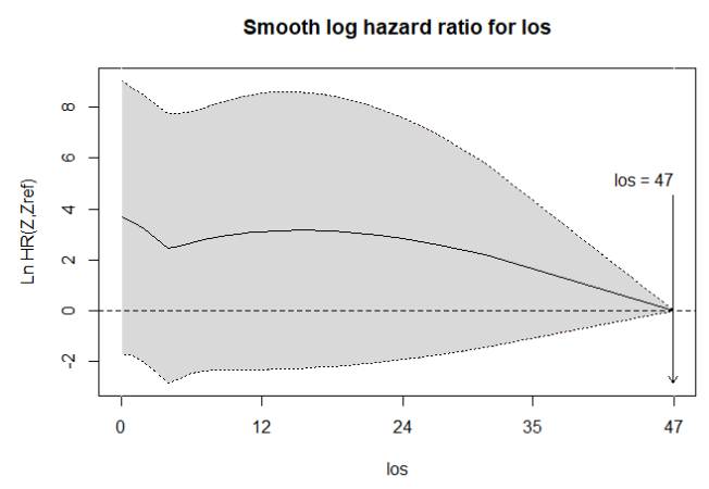
References
Cadarso-Suarez, C. et al. Flexible hazard ratio curves for continuous predictors in multi-state models: an application to breast cancer data. Statistical Modelling, 10(3), 291-314.
Meira-Machado, L. et al. smoothHR: An R Package for Pointwise Nonparametric Estimation of Hazard Ratio Curves of Continuous Predictors. Computational and Mathematical Methods in Medicine, 2013, 11 pages.
