This is a summary blog around "GAMES101: Introduction to Modern Computer Graphics", taught by Lingqi Yan. The knowledge and images involved are quoted from the instructor Lingqi Yan's lecture notes and book "Fundamentals of Computer Graphics 4th".

Catalog

Why Transfromation ?

What are Transformation marices ?

1. 2D Linear transformations

2. Homogenous Coordinates

2.1 Why Homogenous Coordinates ?

2.2 Solution: Homogenous Coordinates !

2.3 Affine Transformations

2.4 2D Transformations in Homogenous Coordinates

3. Inverse Transform

4. Composing and Decomposing Transforms

5. 3D Transformations

5.1 Basic 3D Transformations

5.2 3D Rotations

Reference

Why Transfromation ?

We need to characterize the movement of the model
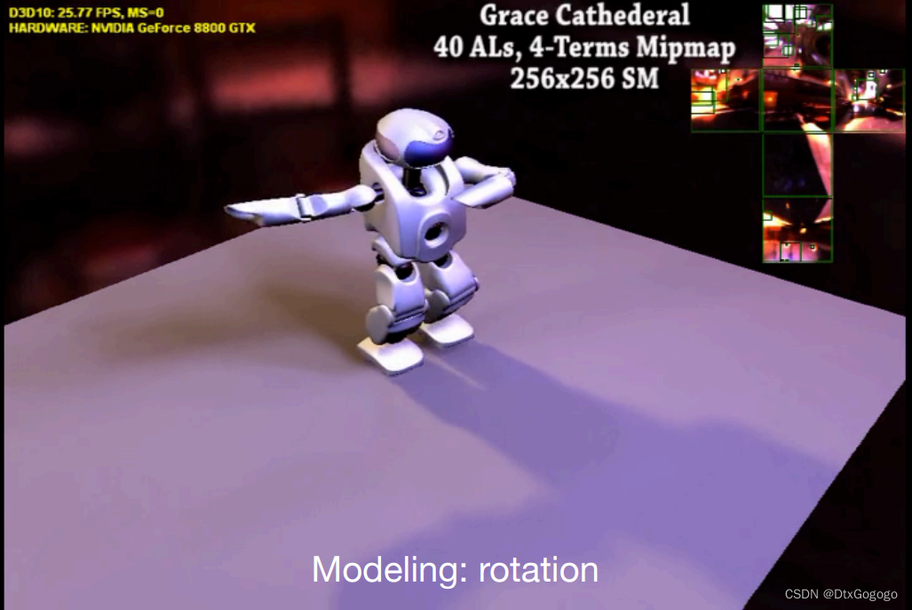
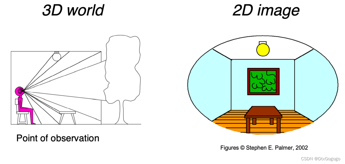
We need to characterize views and projections in different dimensions and from different angles

What are Transformation marices ?

From a mathematical point of view, we can represent the transformations as marices. The importance of transformation marices in graphics needs no introduction. The scaling, rotation, and displacement of all objects can be obtained by transformation marices. There are also many applications in projection transformations, and this article will introduce some brief transformation matrices.

1. 2D Linear transformations

We define the simple matrix(of the same dimension) multiplication shown below as a linear transformation of the vector $\left ( x,y \right )^{T}$ .

$\large \left[\begin{array}{ll} a_{11} & a_{12} \\ a_{21} & a_{22} \end{array}\right]\left[\begin{array}{l} x \\ y \end{array}\right]=\left[\begin{array}{l} a_{11} x+a_{12} y \\ a_{21} x+a_{22} y \end{array}\right]$

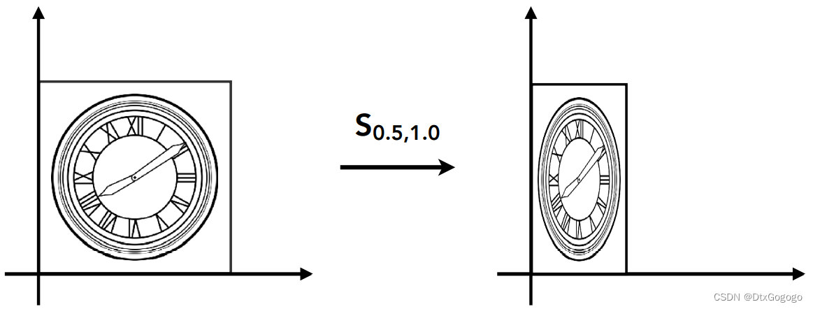
1.1 Scale

The scaling transformation is a transformation that acts along the coordinate axes and is defined as follows,

$\LARGE \left[\begin{array}{l} x^{\prime} \\ y^{\prime} \end{array}\right]=\left[\begin{array}{cc} s_{x} & 0 \\ 0 & s_{y} \end{array}\right]\left[\begin{array}{l} x \\ y \end{array}\right]$

1.2 Reflection

Reflection transformation with a certain coordinate axis as the symmetry axis is defined as follows,

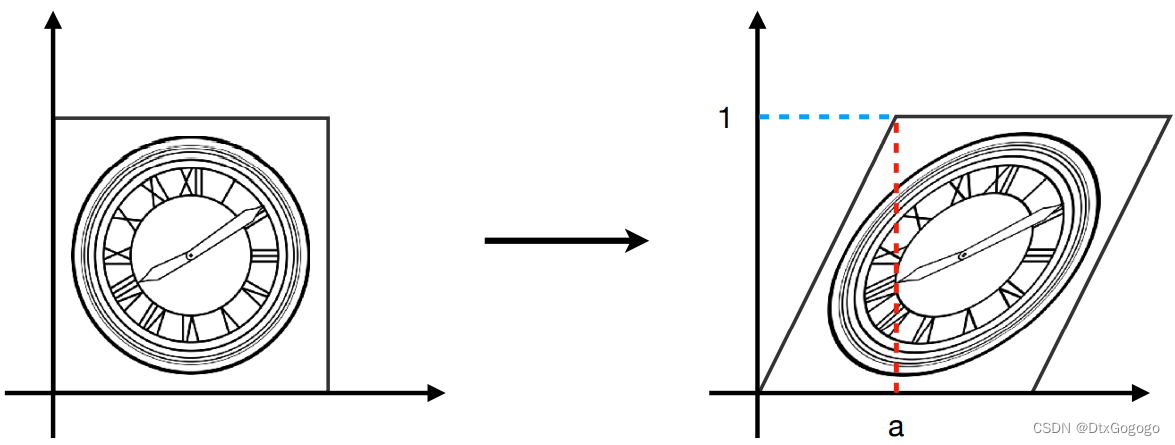
$\LARGE \left[\begin{array}{l} x^{\prime} \\ y^{\prime} \end{array}\right]=\left[\begin{array}{cc} -1 & 0 \\ 0 & 1 \end{array}\right]\left[\begin{array}{l} x \\ y \end{array}\right]$

1.3 Shear

The shear causes a distortion in the image, which is produced in only one direction, i.e., the horizontal shear transformation and the vertical shear transformation, respectively. Horizontal shear transformation is defined as follows,

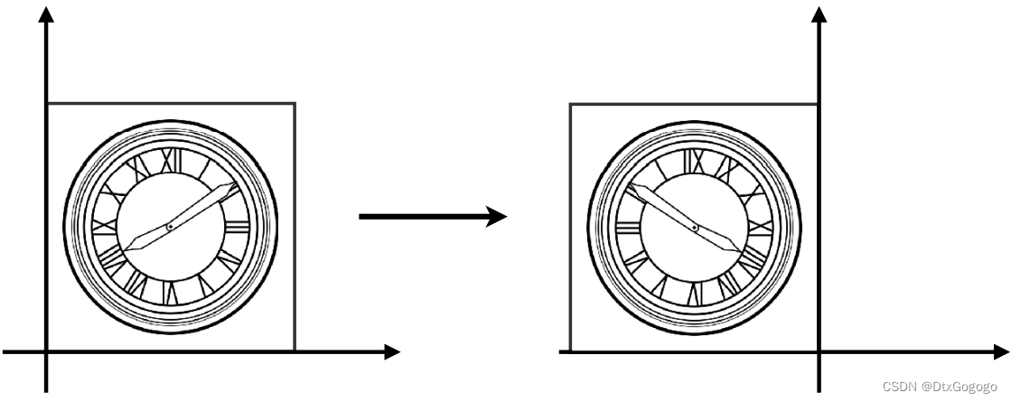
$\LARGE \left[\begin{array}{l} x^{\prime} \\ y^{\prime} \end{array}\right]=\left[\begin{array}{cc} 1 & a \\ 0 & 1 \end{array}\right]\left[\begin{array}{l} x \\ y \end{array}\right]$

1.4 Rotation

Rotation is another very important transformation matrix. We start with the rotation matrix around the origin. In the figure below, we want to represent the rotation of the vector $\LARGE a$ to the vector $\LARGE b$ with a transformation matrix.

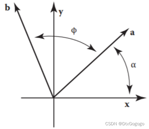
Given that the angle between vector $\LARGE a$ and the $\LARGE x$ -axis is $\LARGE \alpha$ , then the length of vector $\LARGE a$ is $\mathrm{r}=\sqrt{\mathrm{x}_{\alpha}^{2}+\mathrm{y}_{\alpha}^{2}}$ , and the coordinate can be calculated as follows,

$\LARGE \left\{\begin{array}{l} \mathrm{x}_{\alpha}=\mathrm{r} \cos \alpha \\ \mathrm{y}_{\alpha}=\mathrm{r} \sin \alpha \end{array}\right.$

Since the vector $b$ is obtained by rotating the vector $a$ , its length is also $r$ , and the angle between the vector $b$ and the $\LARGE x$ -axis is $\left ( \alpha+\phi \right )$ . It can be obtained using triangle conversion,

$\LARGE \begin{array}{l} \mathrm{x}_{\mathrm{b}}=\mathrm{r} \cos (\alpha+\phi)=\mathrm{r} \cos \alpha \cos \phi-\mathrm{r} \sin \alpha \sin \phi \\ \mathrm{y}_{\mathrm{b}}=\mathrm{r} \sin (\alpha+\phi)=\mathrm{r} \sin \alpha \cos \phi+\mathrm{r} \cos \alpha \sin \phi \end{array}$

Known that $\large \begin{array}{l} \mathrm{x}_{\alpha}=\mathrm{r} \cos \alpha \end{array}$ and $\large \begin{array}{l} \mathrm{y}_{\alpha}=\mathrm{r} \sin \alpha \end{array}$ , the vector $b$ can be rewritten as,

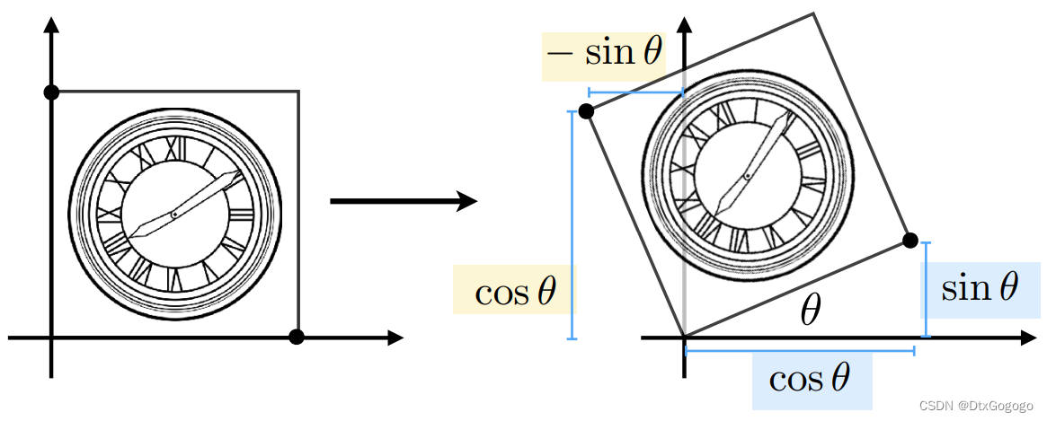
$\LARGE \begin{array}{l} \mathrm{x}_{\mathrm{b}}=\mathrm{x}_{\mathrm{a}} \cos \phi-\mathrm{y}_{\mathrm{a}} \sin \phi \\ \mathrm{y}_{\mathrm{b}}=\mathrm{x}_{\mathrm{a}} \sin \phi+\mathrm{y}_{\mathrm{a}} \cos \phi \end{array}$

The rotational transformation is defined as follows,

$\large \left[\begin{array}{l} \mathrm{x}_{\mathrm{b}} \\ \mathrm{y}_{\mathrm{b}} \end{array}\right]=\left[\begin{array}{cc} \cos \phi & -\sin \phi \\ \sin \phi & \cos \phi \end{array}\right]\left[\begin{array}{l} \mathrm{x}_{\mathrm{a}} \\ \mathrm{y}_{\mathrm{a}} \end{array}\right]$

2. Homogenous Coordinates

2.1 Why Homogenous Coordinates ?

When it comes to translation transformation...

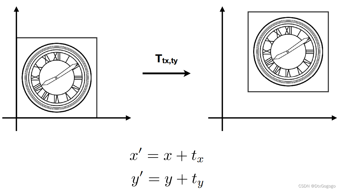
$\large \left[\begin{array}{l} x^{\prime} \\ y^{\prime} \end{array}\right]=\left[\begin{array}{ll} a & b \\ c & d \end{array}\right]\left[\begin{array}{l} x \\ y \end{array}\right]+\left[\begin{array}{l} t_{x} \\ t_{y} \end{array}\right]$

Translation cannot be represented in matrix form.
But we don’t want translation to be a special case. Is there a unified way to represent all transformations? (and what’s the cost?)

2.2 Solution: Homogenous Coordinates !

In order to define the translation transformations as transformation matrices, we add a third coordinate (w-coordinate),

2D point = $\large (x,y,1)^{T}$

2D vector = $\large (x,y,0)^{T}$

Matrix representation of translations,

$\LARGE \left(\begin{array}{c} x^{\prime} \\ y^{\prime} \\ w^{\prime} \end{array}\right)=\left(\begin{array}{ccc} 1 & 0 & t_{x} \\ 0 & 1 & t_{y} \\ 0 & 0 & 1 \end{array}\right) \cdot\left(\begin{array}{l} x \\ y \\ 1 \end{array}\right)=\left(\begin{array}{c} x+t_{x} \\ y+t_{y} \\ 1 \end{array}\right)$

Valid operation if w-coordinate of result is 1 or 0

$\large vector+vector=vector$

$\large point-point=vector$

$\large point+vector=vector$

In homogeneous coordinates, $\large (x,y,w)^{T}$ is the 2D point $\large (x/w,y/w,1)^{T}, w\neq 0$ .

2.3 Affine Transformations

Affine map = linear map + translation

$\large \left(\begin{array}{l} x^{\prime} \\ y^{\prime} \end{array}\right)=\left(\begin{array}{ll} a & b \\ c & d \end{array}\right) \cdot\left(\begin{array}{l} x \\ y \end{array}\right)+\left(\begin{array}{l} t_{x} \\ t_{y} \end{array}\right)$

Using homogenous coordinates, it can be defined as follows,

$\large \left(\begin{array}{c} x^{\prime} \\ y^{\prime} \\ 1 \end{array}\right)=\left(\begin{array}{lll} a & b & t_{x} \\ c & d & t_{y} \\ 0 & 0 & 1 \end{array}\right) \cdot\left(\begin{array}{l} x \\ y \\ 1 \end{array}\right)$

Note: "Affine map = linear map + translation" means it perform linear transformation first and then translation transformation.

2.4 2D Transformations in Homogenous Coordinates

Scale

$\large \mathbf{S}\left(s_{x}, s_{y}\right)=\left(\begin{array}{ccc} s_{x} & 0 & 0 \\ 0 & s_{y} & 0 \\ 0 & 0 & 1 \end{array}\right)$

Rotation by angle α around the origin

$\large \mathbf{R}(\alpha)=\left(\begin{array}{ccc} \cos \alpha & -\sin \alpha & 0 \\ \sin \alpha & \cos \alpha & 0 \\ 0 & 0 & 1 \end{array}\right)$

Translation

$\large \mathbf{T}\left(t_{x}, t_{y}\right)=\left(\begin{array}{ccc} 1 & 0 & t_{x} \\ 0 & 1 & t_{y} \\ 0 & 0 & 1 \end{array}\right)$

3. Inverse Transform

$M^{-1}$ is the inverse of $M$ transform in both a matrix and geometric sense

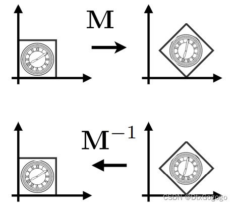
The transformation matrix of the rotation is an orthogonal matrix, so the inverse matrix can be obtained by transposing. In other words, we can transpose a rotation transformation matrix to get its inverse transformation matrix.

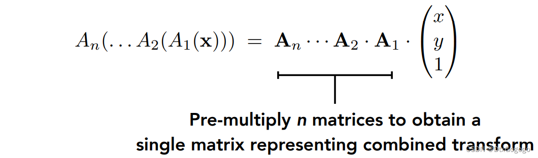
4. Composing and Decomposing Transforms

A sequence of affine transforms can be composed to one transformation matrix by matrix multiplication. Note that matrices are applied right to left.

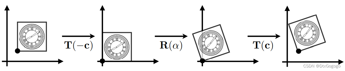
A complex transformation can also be split into multiple simple transformations. For example, when we need to rotate around a given point c,

$\large R_{(c,\alpha)}=T(c )\cdot R(\alpha )\cdot T(-c )$

5. 3D Transformations

Use homogeneous coordinates again,

3D point = $\large (x,y,z,1)^T$

3D vector = $\large (x,y,z,0)^T$

Use 4×4 matrices for affine transformations,

$\large \left(\begin{array}{l} x^{\prime} \\ y^{\prime} \\ z^{\prime} \\ 1 \end{array}\right)=\left(\begin{array}{lllc} a & b & c & t_{x} \\ d & e & f & t_{y} \\ g & h & i & t_{z} \\ 0 & 0 & 0 & 1 \end{array}\right) \cdot\left(\begin{array}{c} x \\ y \\ z \\ 1 \end{array}\right)$

5.1 Basic 3D Transformations

Scale

$\large \mathbf{S}\left(s_{x}, s_{y}, s_{z}\right)=\left(\begin{array}{cccc} s_{x} & 0 & 0 & 0 \\ 0 & s_{y} & 0 & 0 \\ 0 & 0 & s_{z} & 0 \\ 0 & 0 & 0 & 1 \end{array}\right)$

Translation

$\large \mathbf{T}\left(t_{x}, t_{y}, t_{z}\right)=\left(\begin{array}{cccc} 1 & 0 & 0 & t_{x} \\ 0 & 1 & 0 & t_{y} \\ 0 & 0 & 1 & t_{z} \\ 0 & 0 & 0 & 1 \end{array}\right)$

Rotation by angle α around x-, y-, or z-axis

$\large \begin{array}{l} \mathbf{R}_{x}(\alpha)=\left(\begin{array}{cccc} 1 & 0 & 0 & 0 \\ 0 & \cos \alpha & -\sin \alpha & 0 \\ 0 & \sin \alpha & \cos \alpha & 0 \\ 0 & 0 & 0 & 1 \end{array}\right) \end{array}$

$\large \begin{array}{l} \mathbf{R}_{y}(\alpha)=\left(\begin{array}{cccc} \cos \alpha & 0 & \sin \alpha & 0 \\ 0 & 1 & 0 & 0 \\ -\sin \alpha & 0 & \cos \alpha & 0 \\ 0 & 0 & 0 & 1 \end{array}\right) \end{array}$

$\large \begin{array}{l} \mathbf{R}_{z}(\alpha)=\left(\begin{array}{cccc} \cos \alpha & -\sin \alpha & 0 & 0 \\ \sin \alpha & \cos \alpha & 0 & 0 \\ 0 & 0 & 1 & 0 \\ 0 & 0 & 0 & 1 \end{array}\right) \end{array}$

Rotation by angle α around n-axis (Rodrigues’ Rotation Formula)

$\large \vec{n}=(n_{x},n_{y},n_{z})$

$\large \mathbf{R}(\mathbf{n}, \alpha)=\cos (\alpha) \mathbf{I}+(1-\cos (\alpha)) \mathbf{n} \mathbf{n}^{T}+\sin (\alpha) \underbrace{\left(\begin{array}{ccc} 0 & -n_{z} & n_{y} \\ n_{z} & 0 & -n_{x} \\ -n_{y} & n_{x} & 0 \end{array}\right)}_{\mathbf{N}}$

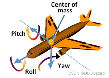
5.2 3D Rotations

Compose any 3D rotation from x-, y-, or z-axis

$\large \mathbf{R}_{x y z}(\alpha, \beta, \gamma)=\mathbf{R}_{x}(\alpha) \mathbf{R}_{y}(\beta) \mathbf{R}_{z}(\gamma)$

Reference

[1] Marschner S , Shirley P. Fundamentals of Computer Graphics 4th

[2] Lingqi Yan, GAMES101: 现代计算机图形学入门

本文含有隐藏内容，请开通VIP 后查看

CG01：Model Transformation In Computer Graphics

Catalog

Why Transfromation ?

What are Transformation marices ?

1. 2D Linear transformations

1.1 Scale

1.2 Reflection

1.3 Shear

1.4 Rotation

2. Homogenous Coordinates

2.1 Why Homogenous Coordinates ?

2.2 Solution: Homogenous Coordinates !

2.3 Affine Transformations

2.4 2D Transformations in Homogenous Coordinates

3. Inverse Transform

4. Composing and Decomposing Transforms

5. 3D Transformations

5.1 Basic 3D Transformations

5.2 3D Rotations

Reference

网站公告

今日签到

热门文章

最新发布