目录
六、线性回归模型的梯度下降算法过程实验(C1_W1_Lab05_Gradient_Descent_Soln)
1.导入使用工具包numpy、matplotlib.pyplot和绘图模块lab_utils_uni
(3).对具体的数据集和初始w,b代入上面的 gradient_descent 函数
看本文前请先阅读专栏内容:“二、线性回归模型”,前文链接如下
一、问题-找到使代价J(w,b)最小的w和b
根据J(w,b)找到使J最小的w和b,这里w和b并不是唯一的

注意:梯度下降法并不只适用于线性回归模型,还广泛应用于深度学习算法

下山的过程就是梯度下降的过程,在每一步都找当前的最速下降方式,但是选择什么初始值(w和b)对梯度下降算法训练也就是选择什么方向决定了你可能到达哪个谷底(谷底可能存在多个)
二、梯度下降算法

这里 学习率α 决定着“下坡”的速度,过快了可能会错过寻找最佳位置(甚至永远都找不到最佳),过慢可能会导致收敛速度慢,后面会提出怎么选择合适的学习率。

左边是上述梯度学习算法的正确实现方式(这种实现方式更为自然,因为每一个w、b对应一个J(w,b),更新的时候要使用当前J(w,b)对应的w和b),右边不是正确的。
三、梯度下降直观理解

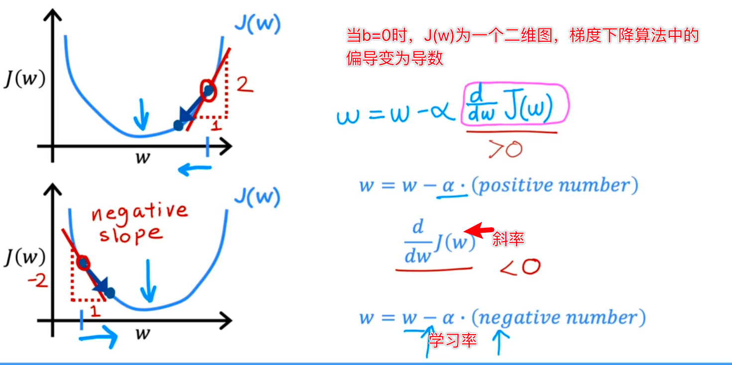
可以先来看w的变化过程,暂时不考虑b,来看为什么w的更新公式会不断地找到令J(w)最小的w:
以标注点为例,斜率<0,w-(斜率),w增大,直至斜率为0,w不变,此时J(w)到达最小值。
四、学习率
前面提到过大或者过小都会有弊端,下面图示解释一下:

下面展示了无论学习率α取多少时,只要J(w)到达局部最小值时,w将不再更新,因为后面紫色部分变为0

下图展示了相同学习率情况下斜率变缓,对w的更新变化(△w)也越来越小,直到到达局部最小值J(w):

五、线性回归中的梯度下降

吴恩达老师对代价函数求偏导代入梯度下降算法的过程(这课程讲的是真的详细):

事实证明,在线性回归模型中的代价函数中,永远不会有多个局部最小值,只有一个全局最小值:

六、线性回归模型的梯度下降算法过程实验(C1_W1_Lab05_Gradient_Descent_Soln)
本实验使用梯度下降法实现了w、b参数的更新变化过程,最终使J(w,b)到达最小值
1.导入使用工具包numpy、matplotlib.pyplot和绘图模块lab_utils_uni
import math, copy
import numpy as np
import matplotlib.pyplot as plt
plt.style.use('./deeplearning.mplstyle')
from lab_utils_uni import plt_house_x, plt_contour_wgrad, plt_divergence, plt_gradients
2.引入数据集

# Load our data set
x_train = np.array([1.0, 2.0])   #features
y_train = np.array([300.0, 500.0])   #target value
3.代码实现代价计算函数 compute_cost

#Function to calculate the cost
def compute_cost(x, y, w, b):

    m = x.shape[0]
    cost = 0

    for i in range(m):
        f_wb = w * x[i] + b
        cost = cost + (f_wb - y[i])**2
    total_cost = 1 / (2 * m) * cost


    return total_cost
4.梯度下降在线性回归模型中应用

(1).计算梯度(代码实现计算上面两个偏导数)
def compute_gradient(x, y, w, b):
    """
    Computes the gradient for linear regression
    Args:
      x (ndarray (m,)): Data, m examples
      y (ndarray (m,)): target values
      w,b (scalar)    : model parameters
    Returns
      dj_dw (scalar): The gradient of the cost w.r.t. the parameters w
      dj_db (scalar): The gradient of the cost w.r.t. the parameter b
     """

    # Number of training examples
    m = x.shape[0]
    dj_dw = 0
    dj_db = 0

    for i in range(m):
        f_wb = w * x[i] + b
        dj_dw_i = (f_wb - y[i]) * x[i]
        dj_db_i = f_wb - y[i]
        dj_db += dj_db_i
        dj_dw += dj_dw_i
    dj_dw = dj_dw / m
    dj_db = dj_db / m

    return dj_dw, dj_db
(2).实现梯度下降过程
gradient_descent 传入 compute_cost、compute_gradient 两个计算函数

def gradient_descent(x, y, w_in, b_in, alpha, num_iters, cost_function, gradient_function):
    """
    Performs gradient descent to fit w,b. Updates w,b by taking
    num_iters gradient steps with learning rate alpha

    Args:
      x (ndarray (m,))  : Data, m examples
      y (ndarray (m,))  : target values
      w_in,b_in (scalar): initial values of model parameters
      alpha (float):     Learning rate
      num_iters (int):   number of iterations to run gradient descent
      cost_function:     function to call to produce cost
      gradient_function: function to call to produce gradient

    Returns:
      w (scalar): Updated value of parameter after running gradient descent
      b (scalar): Updated value of parameter after running gradient descent
      J_history (List): History of cost values
      p_history (list): History of parameters [w,b]
      """

    w = copy.deepcopy(w_in) # avoid modifying global w_in
    # An array to store cost J and w's at each iteration primarily for graphing later
    J_history = []
    p_history = []
    b = b_in
    w = w_in

    for i in range(num_iters):
        # Calculate the gradient and update the parameters using gradient_function
        dj_dw, dj_db = gradient_function(x, y, w , b)

        # Update Parameters using equation (3) above
        b = b - alpha * dj_db
        w = w - alpha * dj_dw

        # Save cost J at each iteration
        if i<100000:      # prevent resource exhaustion
            J_history.append( cost_function(x, y, w , b))
            p_history.append([w,b])
        # Print cost every at intervals 10 times or as many iterations if < 10
        if i% math.ceil(num_iters/10) == 0:
            print(f"Iteration {i:4}: Cost {J_history[-1]:0.2e} ",
                  f"dj_dw: {dj_dw: 0.3e}, dj_db: {dj_db: 0.3e}  ",
                  f"w: {w: 0.3e}, b:{b: 0.5e}")

    return w, b, J_history, p_history #return w and J,w history for graphing
(3).对具体的数据集和初始w,b代入上面的 gradient_descent 函数
# initialize parameters
w_init = 0
b_init = 0
# some gradient descent settings
iterations = 10000
tmp_alpha = 1.0e-2
# run gradient descent
w_final, b_final, J_hist, p_hist = gradient_descent(x_train ,y_train, w_init, b_init, tmp_alpha,
                                                    iterations, compute_cost, compute_gradient)
print(f"(w,b) found by gradient descent: ({w_final:8.4f},{b_final:8.4f})")迭代执行10000次后执行结果:(△w的变化越来越缓,趋势看“四、学习率”的最后一图)

注:代价与迭代次数的关系图是衡量梯度下降法进展的一个有用指标。在成功的运行中,代价Cost总是会降低。代价Cost的变化在一开始是如此迅速,所以用不同的尺度绘制初始下降曲线和最终下降曲线是很有用的。在下面的图中,注意坐标轴上的代价Cost规模和迭代步骤。
# plot cost versus iteration
fig, (ax1, ax2) = plt.subplots(1, 2, constrained_layout=True, figsize=(12,4))
ax1.plot(J_hist[:100])
ax2.plot(1000 + np.arange(len(J_hist[1000:])), J_hist[1000:])
ax1.set_title("Cost vs. iteration(start)");  ax2.set_title("Cost vs. iteration (end)")
ax1.set_ylabel('Cost')            ;  ax2.set_ylabel('Cost')
ax1.set_xlabel('iteration step')  ;  ax2.set_xlabel('iteration step')
plt.show()
(4).预测
用上面得到的w和b代入线性回归模型进行预测
print(f"1000 sqft house prediction {w_final*1.0 + b_final:0.1f} Thousand dollars")
print(f"1200 sqft house prediction {w_final*1.2 + b_final:0.1f} Thousand dollars")
print(f"2000 sqft house prediction {w_final*2.0 + b_final:0.1f} Thousand dollars")
(5).高学习率的情况 α=0.8 时
# initialize parameters
w_init = 0
b_init = 0
# set alpha to a large value
iterations = 10
tmp_alpha = 8.0e-1
# run gradient descent
w_final, b_final, J_hist, p_hist = gradient_descent(x_train ,y_train, w_init, b_init, tmp_alpha,
                                                    iterations, compute_cost, compute_gradient)
迭代更快,但是出现了Cost不降反增的情况:

上面左图显示了w在梯度下降的前几个步骤中的进展。w从正到负波动,成本增长迅速。梯度下降同时作用于w和b,右侧的3D图能获得完整的图像。
下一章将学习——多元变量的线性回归模型