注意力可视化
训练模型
包含通道注意力模块和CNN模型的定义(通道注意力的插入)
import torch
import torch.nn as nn
import torch.optim as optim
from torchvision import datasets, transforms
from torch.utils.data import DataLoader
import matplotlib.pyplot as plt
import numpy as np
# 设置中文字体支持
plt.rcParams["font.family"] = ["SimHei"]
plt.rcParams['axes.unicode_minus'] = False # 解决负号显示问题
# 检查GPU是否可用
device = torch.device("cuda" if torch.cuda.is_available() else "cpu")
print(f"使用设备: {device}")
# 1. 数据预处理
# 训练集:使用多种数据增强方法提高模型泛化能力
train_transform = transforms.Compose([
# 随机裁剪图像,从原图中随机截取32x32大小的区域
transforms.RandomCrop(32, padding=4),
# 随机水平翻转图像(概率0.5)
transforms.RandomHorizontalFlip(),
# 随机颜色抖动:亮度、对比度、饱和度和色调随机变化
transforms.ColorJitter(brightness=0.2, contrast=0.2, saturation=0.2, hue=0.1),
# 随机旋转图像(最大角度15度)
transforms.RandomRotation(15),
# 将PIL图像或numpy数组转换为张量
transforms.ToTensor(),
# 标准化处理:每个通道的均值和标准差,使数据分布更合理
transforms.Normalize((0.4914, 0.4822, 0.4465), (0.2023, 0.1994, 0.2010))
])
# 测试集:仅进行必要的标准化,保持数据原始特性,标准化不损失数据信息,可还原
test_transform = transforms.Compose([
transforms.ToTensor(),
transforms.Normalize((0.4914, 0.4822, 0.4465), (0.2023, 0.1994, 0.2010))
])
# 2. 加载CIFAR-10数据集
train_dataset = datasets.CIFAR10(
root='./data',
train=True,
download=True,
transform=train_transform # 使用增强后的预处理
)
test_dataset = datasets.CIFAR10(
root='./data',
train=False,
transform=test_transform # 测试集不使用增强
)
# 3. 创建数据加载器
batch_size = 64
train_loader = DataLoader(train_dataset, batch_size=batch_size, shuffle=True)
test_loader = DataLoader(test_dataset, batch_size=batch_size, shuffle=False)
# ===================== 新增:通道注意力模块(SE模块) =====================
class ChannelAttention(nn.Module):
"""通道注意力模块(Squeeze-and-Excitation)"""
def __init__(self, in_channels, reduction_ratio=16):
"""
参数:
in_channels: 输入特征图的通道数
reduction_ratio: 降维比例,用于减少参数量
"""
super(ChannelAttention, self).__init__()
# 全局平均池化 - 将空间维度压缩为1x1,保留通道信息
self.avg_pool = nn.AdaptiveAvgPool2d(1)
# 全连接层 + 激活函数,用于学习通道间的依赖关系
self.fc = nn.Sequential(
# 降维:压缩通道数,减少计算量
nn.Linear(in_channels, in_channels // reduction_ratio, bias=False),
nn.ReLU(inplace=True),
# 升维:恢复原始通道数
nn.Linear(in_channels // reduction_ratio, in_channels, bias=False),
# Sigmoid将输出值归一化到[0,1],表示通道重要性权重
nn.Sigmoid()
)
def forward(self, x):
"""
参数:
x: 输入特征图,形状为 [batch_size, channels, height, width]
返回:
加权后的特征图,形状不变
"""
batch_size, channels, height, width = x.size()
# 1. 全局平均池化:[batch_size, channels, height, width] → [batch_size, channels, 1, 1]
avg_pool_output = self.avg_pool(x)
# 2. 展平为一维向量:[batch_size, channels, 1, 1] → [batch_size, channels]
avg_pool_output = avg_pool_output.view(batch_size, channels)
# 3. 通过全连接层学习通道权重:[batch_size, channels] → [batch_size, channels]
channel_weights = self.fc(avg_pool_output)
# 4. 重塑为二维张量:[batch_size, channels] → [batch_size, channels, 1, 1]
channel_weights = channel_weights.view(batch_size, channels, 1, 1)
# 5. 将权重应用到原始特征图上(逐通道相乘)
return x * channel_weights # 输出形状:[batch_size, channels, height, width]
# 4. 定义CNN模型的定义(通道注意力的插入)
class CNN(nn.Module):
def __init__(self):
super(CNN, self).__init__()
# ---------------------- 第一个卷积块 ----------------------
self.conv1 = nn.Conv2d(3, 32, 3, padding=1)
self.bn1 = nn.BatchNorm2d(32)
self.relu1 = nn.ReLU()
# 新增:插入通道注意力模块(SE模块)
self.ca1 = ChannelAttention(in_channels=32, reduction_ratio=16)
self.pool1 = nn.MaxPool2d(2, 2)
# ---------------------- 第二个卷积块 ----------------------
self.conv2 = nn.Conv2d(32, 64, 3, padding=1)
self.bn2 = nn.BatchNorm2d(64)
self.relu2 = nn.ReLU()
# 新增:插入通道注意力模块(SE模块)
self.ca2 = ChannelAttention(in_channels=64, reduction_ratio=16)
self.pool2 = nn.MaxPool2d(2)
# ---------------------- 第三个卷积块 ----------------------
self.conv3 = nn.Conv2d(64, 128, 3, padding=1)
self.bn3 = nn.BatchNorm2d(128)
self.relu3 = nn.ReLU()
# 新增:插入通道注意力模块(SE模块)
self.ca3 = ChannelAttention(in_channels=128, reduction_ratio=16)
self.pool3 = nn.MaxPool2d(2)
# ---------------------- 全连接层(分类器) ----------------------
self.fc1 = nn.Linear(128 * 4 * 4, 512)
self.dropout = nn.Dropout(p=0.5)
self.fc2 = nn.Linear(512, 10)
def forward(self, x):
# ---------- 卷积块1处理 ----------
x = self.conv1(x)
x = self.bn1(x)
x = self.relu1(x)
x = self.ca1(x) # 应用通道注意力
x = self.pool1(x)
# ---------- 卷积块2处理 ----------
x = self.conv2(x)
x = self.bn2(x)
x = self.relu2(x)
x = self.ca2(x) # 应用通道注意力
x = self.pool2(x)
# ---------- 卷积块3处理 ----------
x = self.conv3(x)
x = self.bn3(x)
x = self.relu3(x)
x = self.ca3(x) # 应用通道注意力
x = self.pool3(x)
# ---------- 展平与全连接层 ----------
x = x.view(-1, 128 * 4 * 4)
x = self.fc1(x)
x = self.relu3(x)
x = self.dropout(x)
x = self.fc2(x)
return x
# 重新初始化模型,包含通道注意力模块
model = CNN()
model = model.to(device) # 将模型移至GPU(如果可用)
criterion = nn.CrossEntropyLoss() # 交叉熵损失函数
optimizer = optim.Adam(model.parameters(), lr=0.001) # Adam优化器
# 引入学习率调度器,在训练过程中动态调整学习率--训练初期使用较大的 LR 快速降低损失,训练后期使用较小的 LR 更精细地逼近全局最优解。
# 在每个 epoch 结束后,需要手动调用调度器来更新学习率,可以在训练过程中调用 scheduler.step()
scheduler = optim.lr_scheduler.ReduceLROnPlateau(
optimizer, # 指定要控制的优化器(这里是Adam)
mode='min', # 监测的指标是"最小化"(如损失函数)
patience=3, # 如果连续3个epoch指标没有改善,才降低LR
factor=0.5 # 降低LR的比例(新LR = 旧LR × 0.5)
)
# 5. 训练模型(记录每个 iteration 的损失)
def train(model, train_loader, test_loader, criterion, optimizer, scheduler, device, epochs):
model.train() # 设置为训练模式
# 记录每个 iteration 的损失
all_iter_losses = [] # 存储所有 batch 的损失
iter_indices = [] # 存储 iteration 序号
# 记录每个 epoch 的准确率和损失
train_acc_history = []
test_acc_history = []
train_loss_history = []
test_loss_history = []
for epoch in range(epochs):
running_loss = 0.0
correct = 0
total = 0
for batch_idx, (data, target) in enumerate(train_loader):
data, target = data.to(device), target.to(device) # 移至GPU
optimizer.zero_grad() # 梯度清零
output = model(data) # 前向传播
loss = criterion(output, target) # 计算损失
loss.backward() # 反向传播
optimizer.step() # 更新参数
# 记录当前 iteration 的损失
iter_loss = loss.item()
all_iter_losses.append(iter_loss)
iter_indices.append(epoch * len(train_loader) + batch_idx + 1)
# 统计准确率和损失
running_loss += iter_loss
_, predicted = output.max(1)
total += target.size(0)
correct += predicted.eq(target).sum().item()
# 每100个批次打印一次训练信息
if (batch_idx + 1) % 100 == 0:
print(f'Epoch: {epoch+1}/{epochs} | Batch: {batch_idx+1}/{len(train_loader)} '
f'| 单Batch损失: {iter_loss:.4f} | 累计平均损失: {running_loss/(batch_idx+1):.4f}')
# 计算当前epoch的平均训练损失和准确率
epoch_train_loss = running_loss / len(train_loader)
epoch_train_acc = 100. * correct / total
train_acc_history.append(epoch_train_acc)
train_loss_history.append(epoch_train_loss)
# 测试阶段
model.eval() # 设置为评估模式
test_loss = 0
correct_test = 0
total_test = 0
with torch.no_grad():
for data, target in test_loader:
data, target = data.to(device), target.to(device)
output = model(data)
test_loss += criterion(output, target).item()
_, predicted = output.max(1)
total_test += target.size(0)
correct_test += predicted.eq(target).sum().item()
epoch_test_loss = test_loss / len(test_loader)
epoch_test_acc = 100. * correct_test / total_test
test_acc_history.append(epoch_test_acc)
test_loss_history.append(epoch_test_loss)
# 更新学习率调度器
scheduler.step(epoch_test_loss)
print(f'Epoch {epoch+1}/{epochs} 完成 | 训练准确率: {epoch_train_acc:.2f}% | 测试准确率: {epoch_test_acc:.2f}%')
# 绘制所有 iteration 的损失曲线
plot_iter_losses(all_iter_losses, iter_indices)
# 绘制每个 epoch 的准确率和损失曲线
plot_epoch_metrics(train_acc_history, test_acc_history, train_loss_history, test_loss_history)
return epoch_test_acc # 返回最终测试准确率
# 6. 绘制每个 iteration 的损失曲线
def plot_iter_losses(losses, indices):
plt.figure(figsize=(10, 4))
plt.plot(indices, losses, 'b-', alpha=0.7, label='Iteration Loss')
plt.xlabel('Iteration(Batch序号)')
plt.ylabel('损失值')
plt.title('每个 Iteration 的训练损失')
plt.legend()
plt.grid(True)
plt.tight_layout()
plt.show()
# 7. 绘制每个 epoch 的准确率和损失曲线
def plot_epoch_metrics(train_acc, test_acc, train_loss, test_loss):
epochs = range(1, len(train_acc) + 1)
plt.figure(figsize=(12, 4))
# 绘制准确率曲线
plt.subplot(1, 2, 1)
plt.plot(epochs, train_acc, 'b-', label='训练准确率')
plt.plot(epochs, test_acc, 'r-', label='测试准确率')
plt.xlabel('Epoch')
plt.ylabel('准确率 (%)')
plt.title('训练和测试准确率')
plt.legend()
plt.grid(True)
# 绘制损失曲线
plt.subplot(1, 2, 2)
plt.plot(epochs, train_loss, 'b-', label='训练损失')
plt.plot(epochs, test_loss, 'r-', label='测试损失')
plt.xlabel('Epoch')
plt.ylabel('损失值')
plt.title('训练和测试损失')
plt.legend()
plt.grid(True)
plt.tight_layout()
plt.show()
# 训练模型(复用原有的train函数)
print("开始训练带通道注意力的CNN模型...")
final_accuracy = train(model, train_loader, test_loader, criterion, optimizer, scheduler, device, epochs=20)
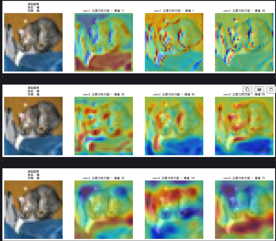
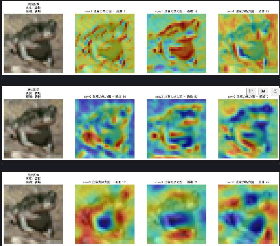
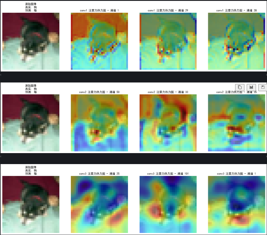
print(f"训练完成!最终测试准确率: {final_accuracy:.2f}%")可视化空间注意力热力图
对比conv1,conv2,conv3这三个卷积层
# 可视化空间注意力热力图(显示模型关注的图像区域)
def visualize_attention_map(model, test_loader, device, class_names, num_samples=3):
    """可视化模型的注意力热力图,展示模型关注的图像区域"""
    model.eval()  # 设置为评估模式

    with torch.no_grad():
        for i, (images, labels) in enumerate(test_loader):
            if i >= num_samples:  # 只可视化前几个样本
                break

            images, labels = images.to(device), labels.to(device)

            # 为多个卷积层创建钩子
            activation_maps = {}
            conv_layers = ['conv1', 'conv2', 'conv3']

            def hook(module, input, output, layer_name):
                activation_maps[layer_name] = output.cpu()

            # 为每个卷积层注册钩子
            hook_handles = []
            for layer_name in conv_layers:
                layer = getattr(model, layer_name)
                handle = layer.register_forward_hook(lambda m, i, o, name=layer_name: hook(m, i, o, name))
                hook_handles.append(handle)

            # 前向传播,触发钩子
            outputs = model(images)

            # 移除所有钩子
            for handle in hook_handles:
                handle.remove()

            # 获取预测结果
            _, predicted = torch.max(outputs, 1)

            # 获取原始图像
            img = images[0].cpu().permute(1, 2, 0).numpy()
            # 反标准化处理
            img = img * np.array([0.2023, 0.1994, 0.2010]).reshape(1, 1, 3) + np.array([0.4914, 0.4822, 0.4465]).reshape(1, 1, 3)
            img = np.clip(img, 0, 1)

            # 为每个卷积层创建子图
            for layer_name in conv_layers:
                # 获取激活图(对应卷积层的输出)
                feature_map = activation_maps[layer_name][0].cpu()  # 取第一个样本

                # 计算通道注意力权重(使用SE模块的全局平均池化)
                channel_weights = torch.mean(feature_map, dim=(1, 2))  # [C]

                # 按权重对通道排序
                sorted_indices = torch.argsort(channel_weights, descending=True)

                # 创建子图
                fig, axes = plt.subplots(1, 4, figsize=(16, 4))

                # 显示原始图像
                axes[0].imshow(img)
                axes[0].set_title(f'原始图像\n真实: {class_names[labels[0]]}\n预测: {class_names[predicted[0]]}')
                axes[0].axis('off')

                # 显示前3个最活跃通道的热力图
                for j in range(3):
                    channel_idx = sorted_indices[j]
                    # 获取对应通道的特征图
                    channel_map = feature_map[channel_idx].numpy()
                    # 归一化到[0,1]
                    channel_map = (channel_map - channel_map.min()) / (channel_map.max() - channel_map.min() + 1e-8)

                    # 调整热力图大小以匹配原始图像
                    from scipy.ndimage import zoom
                    heatmap = zoom(channel_map, (32/feature_map.shape[1], 32/feature_map.shape[2]))

                    # 显示热力图
                    axes[j+1].imshow(img)
                    axes[j+1].imshow(heatmap, alpha=0.5, cmap='jet')
                    axes[j+1].set_title(f'{layer_name} 注意力热力图 - 通道 {channel_idx}')
                    axes[j+1].axis('off')

                plt.tight_layout()
                plt.show()

# 调用可视化函数
class_names = ['飞机', '汽车', '鸟', '猫', '鹿', '狗', '青蛙', '马', '船', '卡车']
visualize_attention_map(model, test_loader, device, class_names, num_samples=3)