0 前言

🔥 Hi，大家好，这里是丹成学长的毕设系列文章！

🔥 对毕设有任何疑问都可以问学长哦!

这两年开始，各个学校对毕设的要求越来越高，难度也越来越大… 毕业设计耗费时间，耗费精力，甚至有些题目即使是专业的老师或者硕士生也需要很长时间，所以一旦发现问题，一定要提前准备，避免到后面措手不及，草草了事。

为了大家能够顺利以及最少的精力通过毕设，学长分享优质毕业设计项目，今天要分享的新项目是

🚩 基于卷积神经网络的手写字符识别

🥇学长这里给一个题目综合评分(每项满分5分)

• 难度系数：4分
• 工作量：4分
• 创新点：3分

🧿 选题指导, 项目分享：

https://gitee.com/yaa-dc/BJH/blob/master/gg/cc/README.md

1 简介

该设计学长使用python基于TensorFlow设计手写数字识别算法，并编程实现GUI界面，构建手写数字识别系统。

这是学长做的深度学习demo，大家可以用于毕业设计。

这里学长不会以论文的形式展现，而是以编程实战完成深度学习项目的角度去描述。

项目要求：主要解决的问题是手写数字识别，最终要完成一个识别系统。

设计识别率高的算法，实现快速识别的系统。

2 LeNet-5 模型的介绍

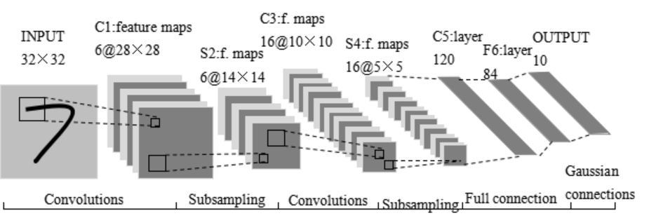
学长实现手写数字识别，使用的是卷积神经网络，建模思想来自LeNet-5，如下图所示：

2.1 结构解析

这是原始的应用于手写数字识别的网络，我认为这也是最简单的深度网络。

LeNet-5不包括输入，一共7层，较低层由卷积层和最大池化层交替构成，更高层则是全连接和高斯连接。

LeNet-5的输入与BP神经网路的不一样。这里假设图像是黑白的，那么LeNet-5的输入是一个32*32的二维矩阵。同
时，输入与下一层并不是全连接的，而是进行稀疏连接。本层每个神经元的输入来自于前一层神经元的局部区域(5×5)，卷积核对原始图像卷积的结果加上相应的阈值，得出的结果再经过激活函数处理，输出即形成卷积层（C层）。卷积层中的每个特征映射都各自共享权重和阈值，这样能大大减少训练开销。降采样层（S层）为减少数据量同时保存有用信息，进行亚抽样。

2.2 C1层

第一个卷积层（C1层）由6个特征映射构成，每个特征映射是一个28×28的神经元阵列，其中每个神经元负责从5×5的区域通过卷积滤波器提取局部特征。一般情况下，滤波器数量越多，就会得出越多的特征映射，反映越多的原始图像的特征。本层训练参数共6×(5×5+1)=156个，每个像素点都是由上层5×5=25个像素点和1个阈值连接计算所得，共28×28×156=122304个连接。

2.3 S2层

S2层是对应上述6个特征映射的降采样层（pooling层）。pooling层的实现方法有两种，分别是max-pooling和mean-pooling，LeNet-5采用的是mean-pooling，即取n×n区域内像素的均值。C1通过2×2的窗口区域像素求均值再加上本层的阈值，然后经过激活函数的处理，得到S2层。pooling的实现，在保存图片信息的基础上，减少了权重参数，降低了计算成本，还能控制过拟合。本层学习参数共有1*6+6=12个，S2中的每个像素都与C1层中的2×2个像素和1个阈值相连，共6×(2×2+1)×14×14=5880个连接。

2.3.1 S2层和C3层连接

S2层和C3层的连接比较复杂。C3卷积层是由16个大小为10×10的特征映射组成的，当中的每个特征映射与S2层的若干个特征映射的局部感受野（大小为5×5）相连。其中，前6个特征映射与S2层连续3个特征映射相连，后面接着的6个映射与S2层的连续的4个特征映射相连，然后的3个特征映射与S2层不连续的4个特征映射相连，最后一个映射与S2层的所有特征映射相连。

此处卷积核大小为5×5，所以学习参数共有6×(3×5×5+1)+9×(4×5×5+1)+1×(6×5×5+1)=1516个参数。而图像大小为28×28，因此共有151600个连接。

S4层是对C3层进行的降采样，与S2同理，学习参数有16×1+16=32个，同时共有16×(2×2+1)×5×5=2000个连接。
C5层是由120个大小为1×1的特征映射组成的卷积层，而且S4层与C5层是全连接的，因此学习参数总个数为120×(16×25+1)=48120个。

2.4 F6与C5层

F6是与C5全连接的84个神经元，所以共有84×(120+1)=10164个学习参数。

卷积神经网络通过通过稀疏连接和共享权重和阈值，大大减少了计算的开销，同时，pooling的实现，一定程度上减少了过拟合问题的出现，非常适合用于图像的处理和识别。

3 写数字识别算法模型的构建

3.1 输入层设计

输入为28×28的矩阵，而不是向量。

3.2 激活函数的选取

Sigmoid函数具有光滑性、鲁棒性和其导数可用自身表示的优点，但其运算涉及指数运算，反向传播求误差梯度时，求导又涉及乘除运算，计算量相对较大。同时，针对本文构建的含有两层卷积层和降采样层，由于sgmoid函数自身的特性，在反向传播时，很容易出现梯度消失的情况，从而难以完成网络的训练。因此，本文设计的网络使用ReLU函数作为激活函数。

3.3 卷积层设计

学长设计卷积神经网络采取的是离散卷积，卷积步长为1，即水平和垂直方向每次运算完，移动一个像素。卷积核大小为5×5。

3.4 降采样层

学长设计的降采样层的pooling方式是max-pooling，大小为2×2。

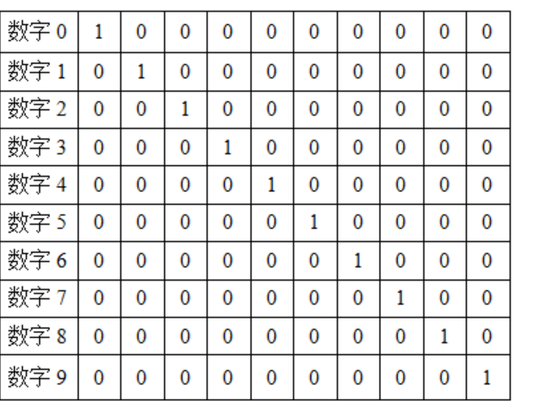
3.5 输出层设计

输出层设置为10个神经网络节点。数字0~9的目标向量如下表所示：

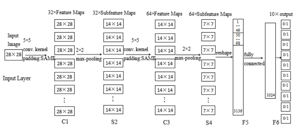
4 网络模型的总体结构

5 部分实现代码

使用Python，调用TensorFlow的api完成手写数字识别的算法。

注：我的程序运行环境是：Win10,python3.。

当然，也可以在Linux下运行，由于TensorFlow对py2和py3兼容得比较好，在Linux下可以在python2.7中运行。

#!/usr/bin/env python2
# -*- coding: utf-8 -*-

#import modules
import numpy as np
import matplotlib.pyplot as plt
#from sklearn.metrics import confusion_matrix
import tensorflow as tf
import time
from datetime import timedelta
import math
from tensorflow.examples.tutorials.mnist import input_data


def new_weights(shape):
  return tf.Variable(tf.truncated_normal(shape,stddev=0.05))
def new_biases(length):
  return tf.Variable(tf.constant(0.1,shape=length))
def conv2d(x,W):
  return tf.nn.conv2d(x,W,strides=[1,1,1,1],padding='SAME')
def max_pool_2x2(inputx):
  return tf.nn.max_pool(inputx,ksize=[1,2,2,1],strides=[1,2,2,1],padding='SAME')

#import data
data = input_data.read_data_sets("./data", one_hot=True) # one_hot means [0 0 1 0 0 0 0 0 0 0] stands for 2

print("Size of:")
print("--Training-set:\t\t{}".format(len(data.train.labels)))
print("--Testing-set:\t\t{}".format(len(data.test.labels)))
print("--Validation-set:\t\t{}".format(len(data.validation.labels)))
data.test.cls = np.argmax(data.test.labels,axis=1)  # show the real test labels: [7 2 1 ..., 4 5 6], 10000values

x = tf.placeholder("float",shape=[None,784],name='x')
x_image = tf.reshape(x,[-1,28,28,1])

y_true = tf.placeholder("float",shape=[None,10],name='y_true')
y_true_cls = tf.argmax(y_true,dimension=1)
# Conv 1
layer_conv1 = {"weights":new_weights([5,5,1,32]),
        "biases":new_biases([32])}
h_conv1 = tf.nn.relu(conv2d(x_image,layer_conv1["weights"])+layer_conv1["biases"])
h_pool1 = max_pool_2x2(h_conv1)
# Conv 2
layer_conv2 = {"weights":new_weights([5,5,32,64]),
        "biases":new_biases([64])}
h_conv2 = tf.nn.relu(conv2d(h_pool1,layer_conv2["weights"])+layer_conv2["biases"])
h_pool2 = max_pool_2x2(h_conv2)
# Full-connected layer 1
fc1_layer = {"weights":new_weights([7*7*64,1024]),
      "biases":new_biases([1024])}
h_pool2_flat = tf.reshape(h_pool2,[-1,7*7*64])
h_fc1 = tf.nn.relu(tf.matmul(h_pool2_flat,fc1_layer["weights"])+fc1_layer["biases"])
# Droupout Layer
keep_prob = tf.placeholder("float")
h_fc1_drop = tf.nn.dropout(h_fc1,keep_prob)
# Full-connected layer 2
fc2_layer = {"weights":new_weights([1024,10]),
       "biases":new_weights([10])}
# Predicted class
y_pred = tf.nn.softmax(tf.matmul(h_fc1_drop,fc2_layer["weights"])+fc2_layer["biases"]) # The output is like [0 0 1 0 0 0 0 0 0 0]
y_pred_cls = tf.argmax(y_pred,dimension=1) # Show the real predict number like '2'
# cost function to be optimized
cross_entropy = -tf.reduce_mean(y_true*tf.log(y_pred))
optimizer = tf.train.AdamOptimizer(learning_rate=1e-4).minimize(cross_entropy)
# Performance Measures
correct_prediction = tf.equal(y_pred_cls,y_true_cls)
accuracy = tf.reduce_mean(tf.cast(correct_prediction,"float"))
with tf.Session() as sess:
  init = tf.global_variables_initializer()
  sess.run(init)
  train_batch_size = 50
  def optimize(num_iterations):
    total_iterations=0
    start_time = time.time()
    for i in range(total_iterations,total_iterations+num_iterations):
      x_batch,y_true_batch = data.train.next_batch(train_batch_size)
      feed_dict_train_op = {x:x_batch,y_true:y_true_batch,keep_prob:0.5}
      feed_dict_train = {x:x_batch,y_true:y_true_batch,keep_prob:1.0}
      sess.run(optimizer,feed_dict=feed_dict_train_op)
      # Print status every 100 iterations.
      if i%100==0:
        # Calculate the accuracy on the training-set.
        acc = sess.run(accuracy,feed_dict=feed_dict_train)
        # Message for printing.
        msg = "Optimization Iteration:{0:>6}, Training Accuracy: {1:>6.1%}"
        # Print it.
        print(msg.format(i+1,acc))
    # Update the total number of iterations performed
    total_iterations += num_iterations
    # Ending time
    end_time = time.time()
    # Difference between start and end_times.
    time_dif = end_time-start_time
    # Print the time-usage
    print("Time usage:"+str(timedelta(seconds=int(round(time_dif)))))
  test_batch_size = 256
  def print_test_accuracy():
    # Number of images in the test-set.
    num_test = len(data.test.images)
    cls_pred = np.zeros(shape=num_test,dtype=np.int)
    i = 0
    while i < num_test:
      # The ending index for the next batch is denoted j.
      j = min(i+test_batch_size,num_test)
      # Get the images from the test-set between index i and j
      images = data.test.images[i:j, :]
      # Get the associated labels
      labels = data.test.labels[i:j, :]
      # Create a feed-dict with these images and labels.
      feed_dict={x:images,y_true:labels,keep_prob:1.0}
      # Calculate the predicted class using Tensorflow.
      cls_pred[i:j] = sess.run(y_pred_cls,feed_dict=feed_dict)
      # Set the start-index for the next batch to the
      # end-index of the current batch
      i = j
    cls_true = data.test.cls
    correct = (cls_true==cls_pred)
    correct_sum = correct.sum()
    acc = float(correct_sum) / num_test
    # Print the accuracy
    msg = "Accuracy on Test-Set: {0:.1%} ({1}/{2})"
    print(msg.format(acc,correct_sum,num_test))
  # Performance after 10000 optimization iterations
  optimize(num_iterations=10000)
  print_test_accuracy()
  savew_hl1 = layer_conv1["weights"].eval()
  saveb_hl1 = layer_conv1["biases"].eval()
  savew_hl2 = layer_conv2["weights"].eval()
  saveb_hl2 = layer_conv2["biases"].eval()
  savew_fc1 = fc1_layer["weights"].eval()
  saveb_fc1 = fc1_layer["biases"].eval()
  savew_op = fc2_layer["weights"].eval()
  saveb_op = fc2_layer["biases"].eval()

  np.save("savew_hl1.npy", savew_hl1)
  np.save("saveb_hl1.npy", saveb_hl1)
  np.save("savew_hl2.npy", savew_hl2)
  np.save("saveb_hl2.npy", saveb_hl2)
  np.save("savew_hl3.npy", savew_fc1)
  np.save("saveb_hl3.npy", saveb_fc1)
  np.save("savew_op.npy", savew_op)
  np.save("saveb_op.npy", saveb_op)

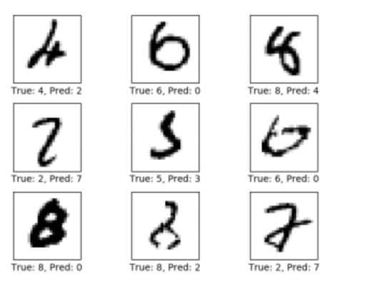
运行结果显示：测试集中准确率大概为99.2%。

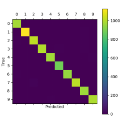
查看混淆矩阵

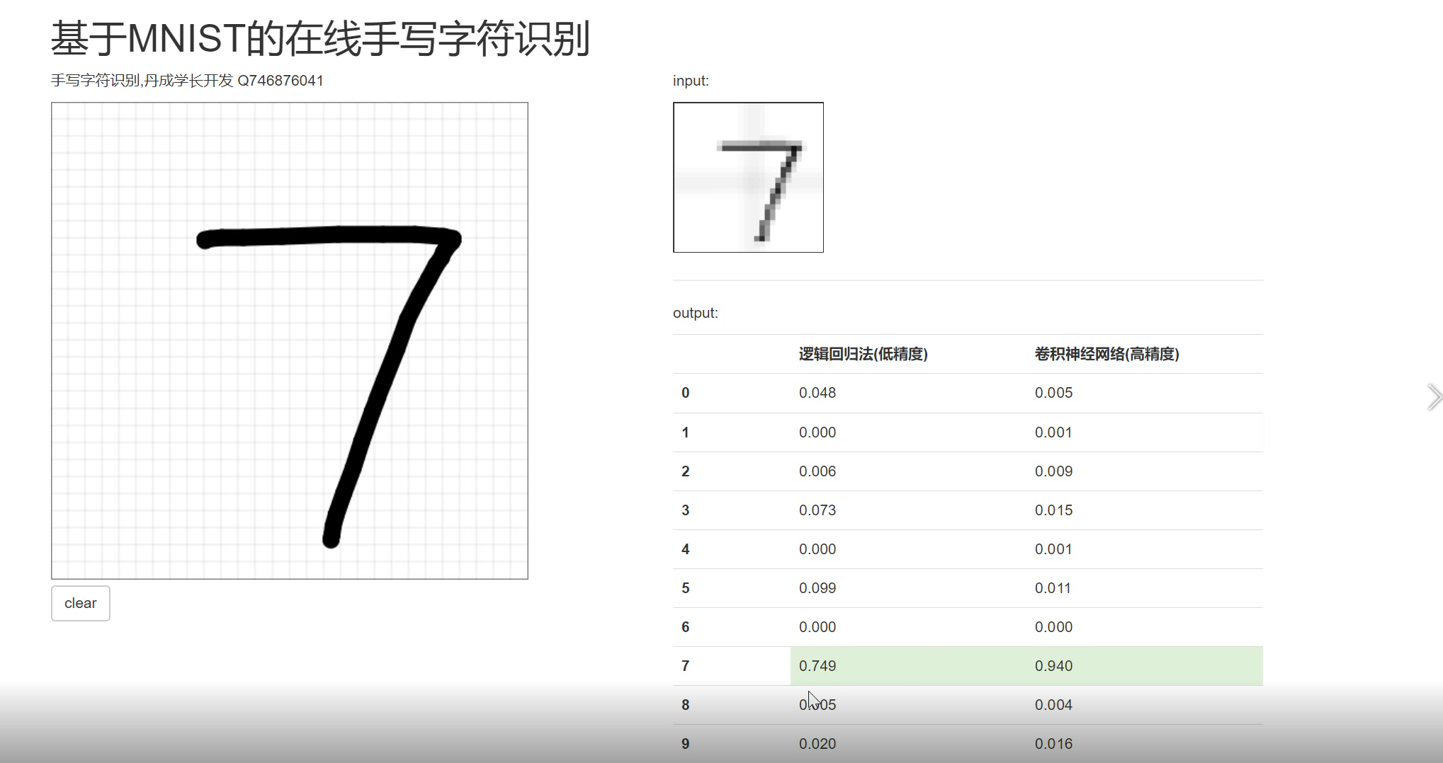
6 在线手写识别

7 最后