李宏毅机器学习 (ML) 课程学习笔记

Some proper nouns（according to the function）

• Regression: outout a scalar. (eg. temperature)
• Classification: given options, and the function outputs the correct one. （eg. chess）
• Structured Learing: create something with structure. (eg. image)

Other nouns (field in ML)

• update: consider the loss process, we need to devide the parameters to many batches, we call the renew of one batch a update;
• epoch: see all the batches once.
• hyperparameter: like learning rate $\eta$, the parameters that ourselves defined.
• overfitting problem: the problems that good in trainning date but bad in predicte date

The process of predict unknow parameters (TRAIN)

We select the linear model to explain.
First step:

• Linear Model: $y=b+w{x}_1$
• w: weight
• b: bias
• lable (the ture number): $\hat{y}$

Second step:

• define loss: L(b, w) = $\frac{1}{N}{\sum }_{n=1}^N{e}_n$,
• normally, $e=|y-\hat{y}|$, L is MAE, normal used;
• normally, $e=(y-\hat{y}{)}^2$, L is MSE
• we need to optimize loss.
• Error Surface: a contour map with w is x-axis, b is y-axis.

The third step: optimization

• $w^{\ast },b^{\ast }=argmi{n}_{w,b}L$
• 解释：在数学优化中，arg min 表示使函数达到最小值时的变量取值. eg. ( arg , min , F(x, y) ) 表示当 ( F(x, y) ) 取得最小值时，变量 ( x, y ) 的取值.
• we use Gradient Descent to optimize, now we only consider one prameter $w$ to show the process.

  • pick a random initial value $w_0$,

  • compute $\frac{\partial L}{\partial w}{|}_{w=w_0}$, then $w_1$ $\leftarrow$ $w_0$ - $\eta \frac{\partial L}{\partial w}{|}_{w=w_0}$.

  • 

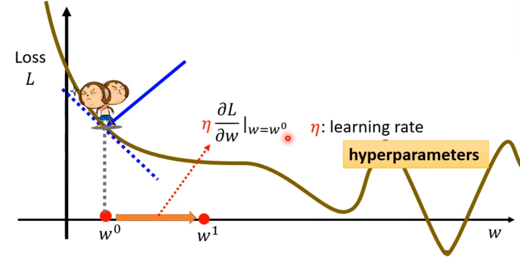
  • update w iteratively.

  • noticed that the gradient descent will cause the problem of local minima, but it's not the main problem.

The condition of other models (Activation function/ Neuron/ Hidden Layer)

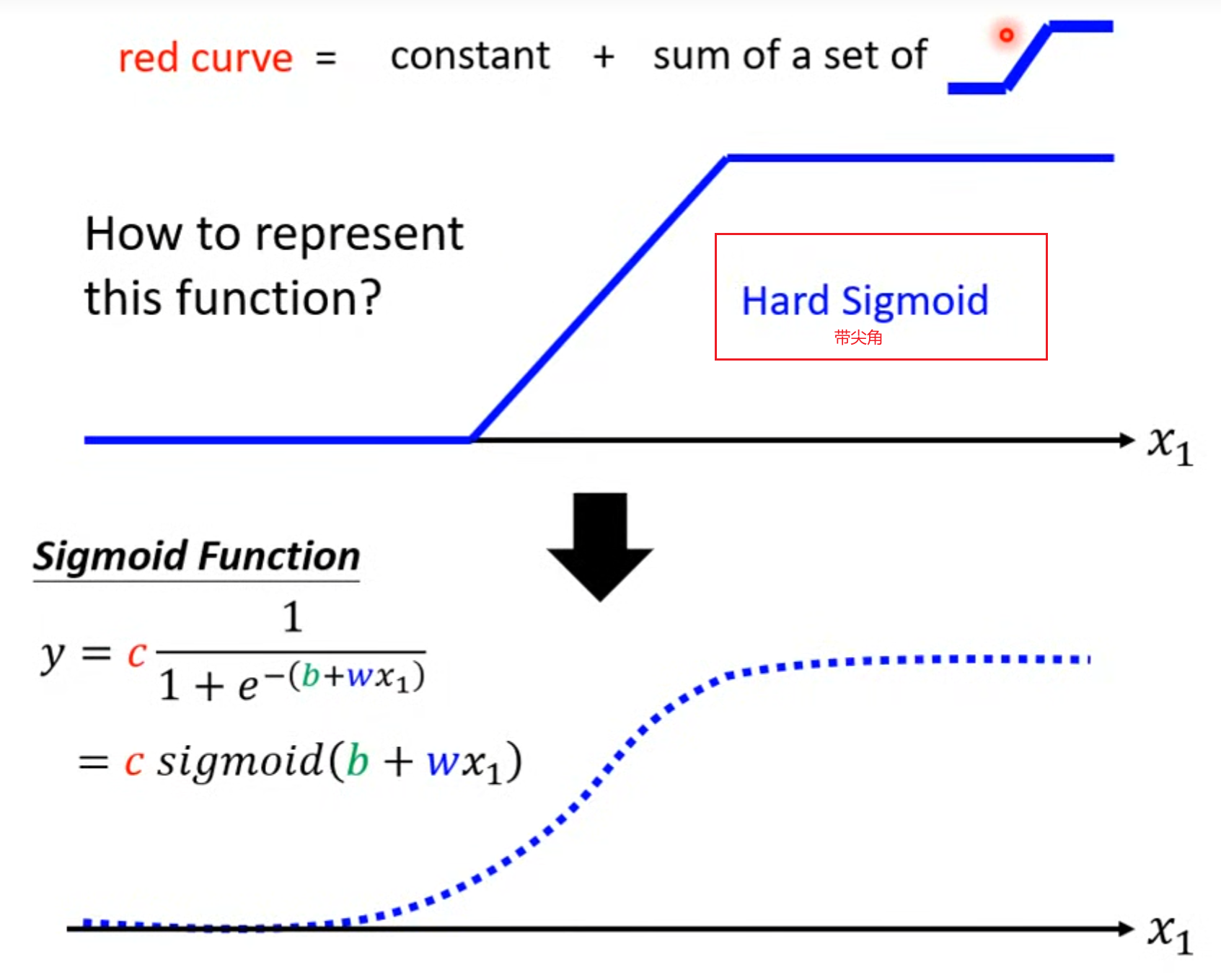
• piecewise linear model = constant + sum of a set of linear model
• y = c $sigmoid(b+w{x}_1)$ = c$\frac{1}{1+e^{-(b+w{x}_1)}}$

  • the featueres of the sigmoid function:

  • 

  • 

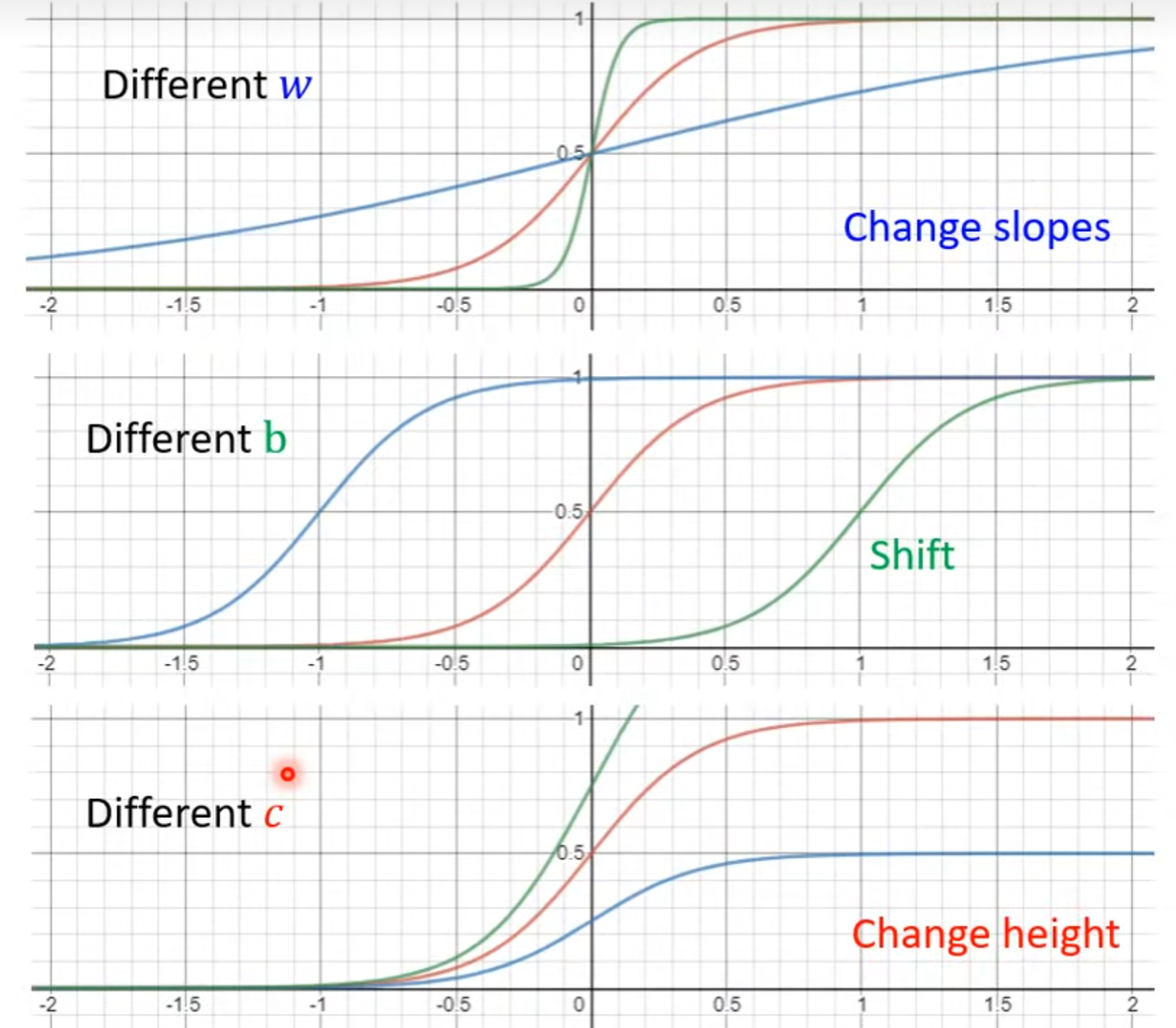
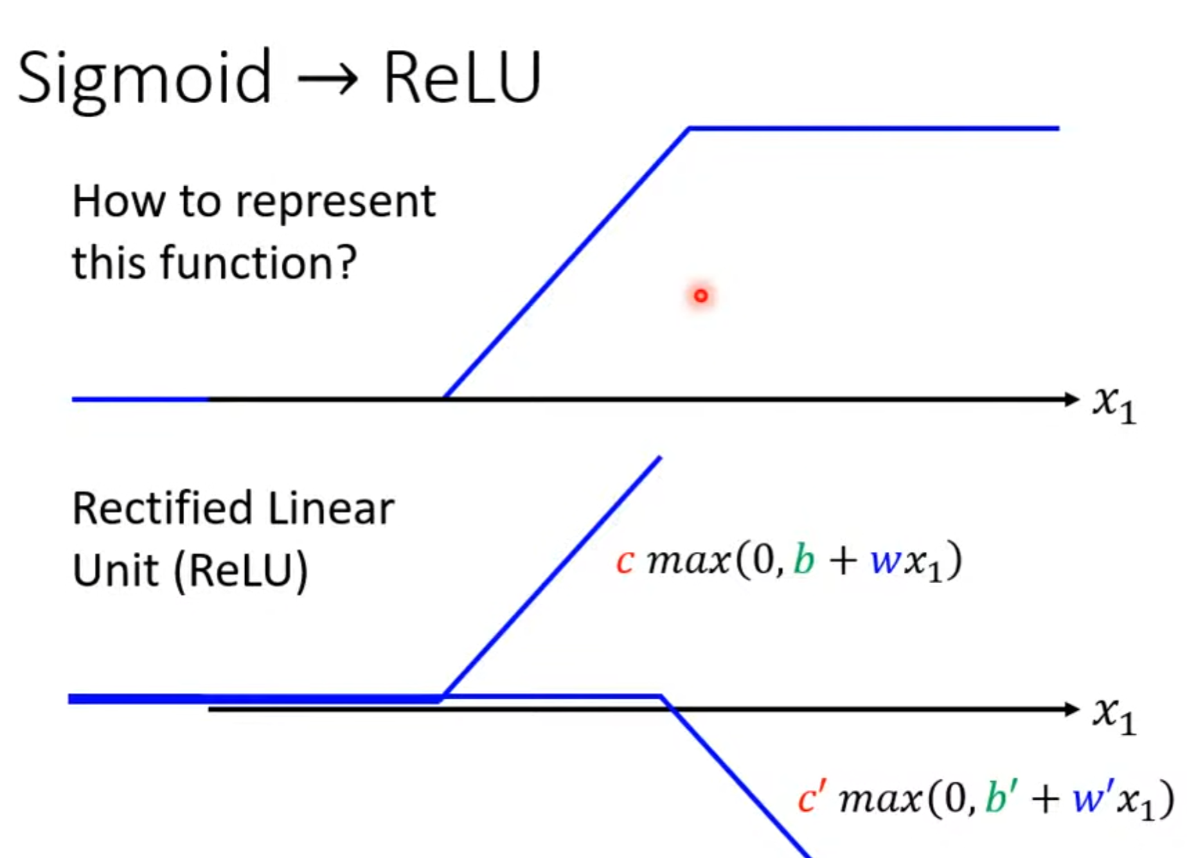
• ReLu: rectified linear unit
  

ATTENTION 1

• About the parameters:
  • model parameters
  • hyperparameters: such as learning rate $\eta$ (in the loss process)

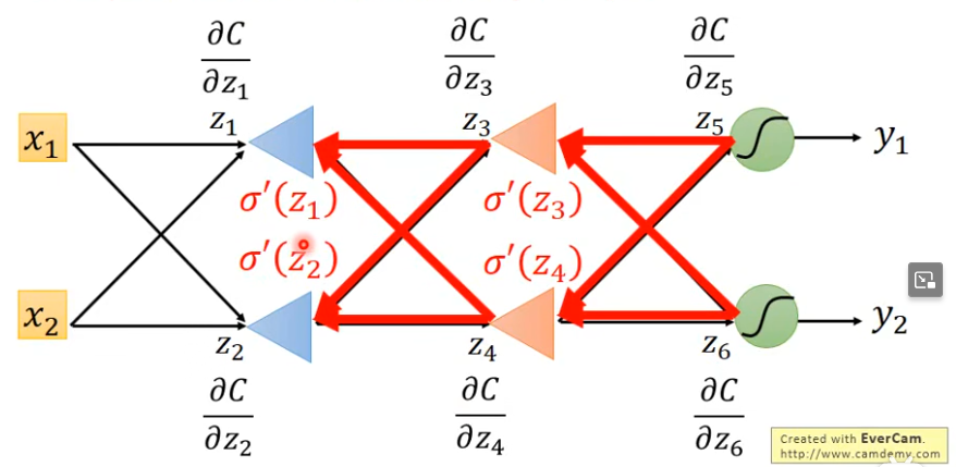
Backpropagation

• an efficient way to compute $\frac{\partial L}{\partial \theta }$. (actually is $\nabla$)
• Chain rule
• generally, we have $\frac{\partial L(\theta )}{\partial w}$ = ${\sum }_{n=1}^N$$\frac{\partial C^n(\theta )}{\partial w}$, where C means one batch of all $\theta s$, so next we should only consider one $\frac{\partial C^n(\theta )}{\partial w}$.
• for one neuron, we have $z=x_1{w}_1+x_2{w}_2+b$
• we have $\frac{\partial C}{\partial w}$ = $\frac{\partial z}{\partial w}$ $\times$ $\frac{\partial C}{\partial z}$= forward pass $\times$ backword pass
• forward pass: $\frac{\partial z}{\partial w}$ = dummy inputs (intuitively obtained )
• backword pass: $\frac{\partial C}{\partial z}$ = $\frac{\partial a}{\partial z}$ $\times$ $\frac{\partial C}{\partial a}$= ${\sigma }^{\prime }(z)[w_3\frac{\partial C}{\partial z^{\prime }}+w_4\frac{\partial C}{\partial z^{\prime \prime }}]$
  • $\frac{\partial a}{\partial z}$ can be intuitively obtained from the above analysis.
  • $\frac{\partial C}{\partial a}$ = $\frac{\partial C}{\partial z^{\prime }}$ $\times$ $\frac{\partial z^{\prime }}{\partial a}$ + $\frac{\partial C}{\partial z^{\prime \prime }}$ $\times$ $\frac{\partial z^{\prime \prime }}{\partial a}$ (the number of z’/z’/… depend on the number of the neurons) = $\frac{\partial y_1}{\partial z^{\prime }}$ $\times$ $\frac{\partial C}{\partial y_1}$ $\times$ $\frac{\partial z^{\prime }}{\partial a}$ + $\frac{\partial y_2}{\partial z^{\prime \prime }}$ $\times$ $\frac{\partial C}{\partial y_2}$ $\times$ $\frac{\partial z^{\prime \prime }}{\partial a}$ (if the layers is end)
  •