目录
一、实现卷积 池化 激活 代码
1、numpy版本
生成图像
图像就是一个矩阵,然后通过一些函数,展示出来。
注:是一个矩阵,不能写数字。(我之前试了试,少写会怎么样,会报错的(TypeError: Image data cannot be converted to float)。)
代码:
import numpy as np
import matplotlib.pyplot as plt


#生成图像
pic = np.array([[-1, -1, -1, -1, -1, -1, -1, -1, -1],
              [-1, 1, -1, -1, -1, -1, -1, 1, -1],
              [-1, -1, 1, -1, -1, -1, 1, -1, -1],
              [-1, -1, -1, 1, -1, 1, -1, -1, -1],
              [-1, -1, -1, -1, 1, -1, -1, -1, -1],
              [-1, -1, -1, 1, -1, 1, -1, -1, -1],
              [-1, -1, 1, -1, -1, -1, 1, -1, -1],
              [-1, 1, -1, -1, -1, -1, -1, 1, -1],
              [-1, -1, -1, -1, -1, -1, -1, -1, -1]])
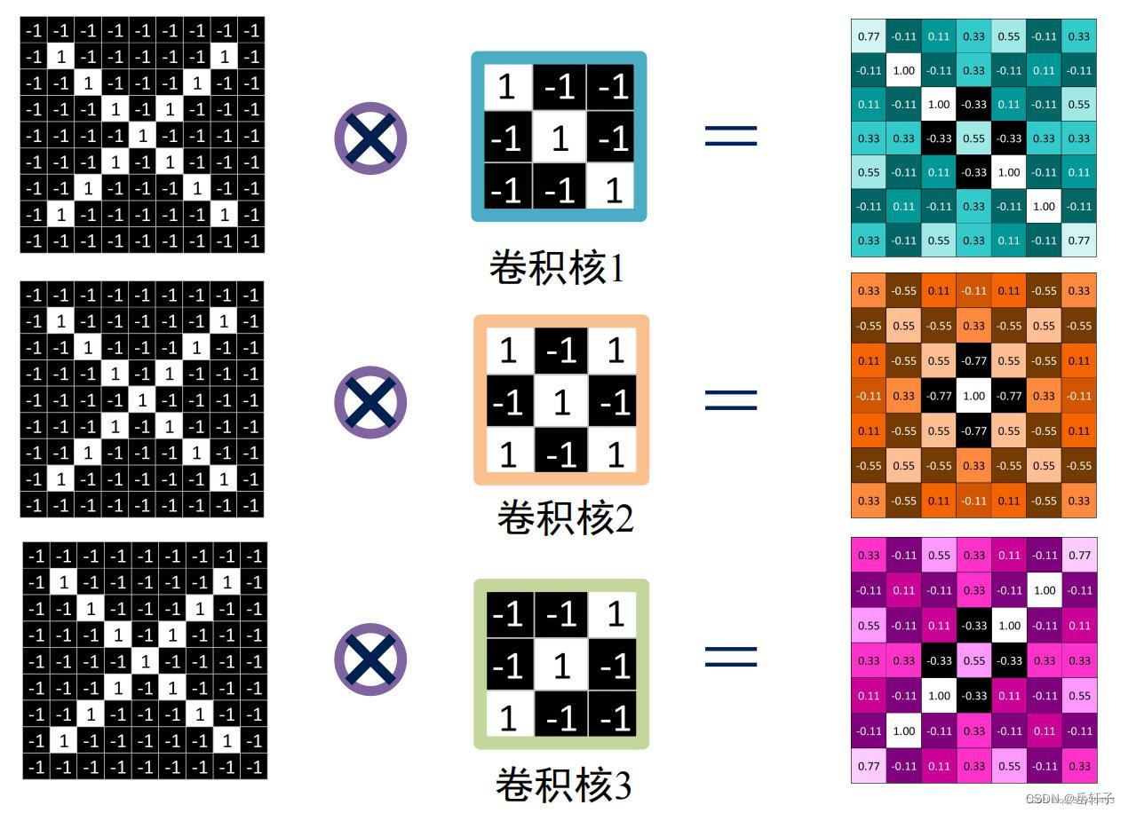
卷积核生成
卷积核就是图像处理时,给定输入图像,输入图像中一个小区域中像素加权平均后成为输出图像中的每个对应像素,其中权值由一个函数定义,这个函数称为卷积核。又称滤波器。
同样提取某个特征,经过不同卷积核卷积后效果也不一样。
一般都是3*3的矩阵
这里初始化三个卷积核
# 初始化三个卷积核

Kernel = [[0 for i in range(0, 3)] for j in range(0, 3)]
Kernel[0] = np.array([[1, -1, -1],
                      [-1, 1, -1],
                      [-1, -1, 1]])
Kernel[1] = np.array([[1, -1, 1],
                      [-1, 1, -1],
                      [1, -1, 1]])
Kernel[2] = np.array([[-1, -1, 1],
                      [-1, 1, -1],
                      [1, -1, -1]])
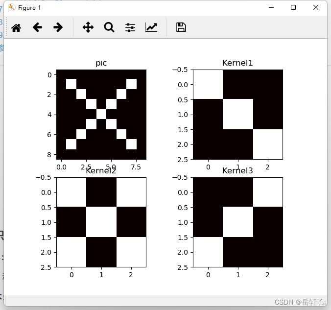
观察一下图像
# 观察原图与卷积核的图像
plt.subplot(221).set_title('pic')
plt.imshow(pic, cmap=plt.cm.hot, vmin=-1, vmax=1)
plt.subplot(222).set_title('Kernel1')
plt.imshow(Kernel[0], cmap=plt.cm.hot, vmin=-1, vmax=1)
plt.subplot(223).set_title('Kernel2')
plt.imshow(Kernel[1], cmap=plt.cm.hot, vmin=-1, vmax=1)
plt.subplot(224).set_title('Kernel3')
plt.imshow(Kernel[2], cmap=plt.cm.hot, vmin=-1, vmax=1)
plt.show()
运行结果:
卷积操作
卷积是分析数学中的一种重要运算,常用于信号处理或图像处理任务。
这里就不多说了,可以看我的上一篇作品
深度学习 实验六 卷积神经网络(1)卷积 torch.nn
手动实现一下(相对于之前有改进):
# 卷积操作
stride = 1  # 步长
feature_map_h = 7  # 特征图的高
feature_map_w = 7  # 特征图的宽
feature_map = [0 for i in range(0, 3)]  # 初始化3个特征图
for i in range(0, 3):
    feature_map[i] = np.zeros((feature_map_h, feature_map_w))  # 初始化特征图
for h in range(feature_map_h):  # 向下滑动,得到卷积后的固定行
    for w in range(feature_map_w):  # 向右滑动,得到卷积后的固定行的列
        v_start = h * stride  # 滑动窗口的起始行(高)
        v_end = v_start + 3  # 滑动窗口的结束行(高)
        h_start = w * stride  # 滑动窗口的起始列(宽)
        h_end = h_start + 3  # 滑动窗口的结束列(宽)
        window = pic[v_start:v_end, h_start:h_end]  # 从图切出一个滑动窗口
        for i in range(0, 3):
            feature_map[i][h, w] = np.divide(np.sum(np.multiply(window, Kernel[i][:, :])), 9)
print("feature_map:\n", np.around(feature_map, decimals=2))
运行结果:
feature_map:
 [[[ 0.78 -0.11  0.11  0.33  0.56 -0.11  0.33]
  [-0.11  1.   -0.11  0.33 -0.11  0.11 -0.11]
  [ 0.11 -0.11  1.   -0.33  0.11 -0.11  0.56]
  [ 0.33  0.33 -0.33  0.56 -0.33  0.33  0.33]
  [ 0.56 -0.11  0.11 -0.33  1.   -0.11  0.11]
  [-0.11  0.11 -0.11  0.33 -0.11  1.   -0.11]
  [ 0.33 -0.11  0.56  0.33  0.11 -0.11  0.78]]

 [[ 0.33 -0.56  0.11 -0.11  0.11 -0.56  0.33]
  [-0.56  0.56 -0.56  0.33 -0.56  0.56 -0.56]
  [ 0.11 -0.56  0.56 -0.78  0.56 -0.56  0.11]
  [-0.11  0.33 -0.78  1.   -0.78  0.33 -0.11]
  [ 0.11 -0.56  0.56 -0.78  0.56 -0.56  0.11]
  [-0.56  0.56 -0.56  0.33 -0.56  0.56 -0.56]
  [ 0.33 -0.56  0.11 -0.11  0.11 -0.56  0.33]]

 [[ 0.33 -0.11  0.56  0.33  0.11 -0.11  0.78]
  [-0.11  0.11 -0.11  0.33 -0.11  1.   -0.11]
  [ 0.56 -0.11  0.11 -0.33  1.   -0.11  0.11]
  [ 0.33  0.33 -0.33  0.56 -0.33  0.33  0.33]
  [ 0.11 -0.11  1.   -0.33  0.11 -0.11  0.56]
  [-0.11  1.   -0.11  0.33 -0.11  0.11 -0.11]
  [ 0.78 -0.11  0.11  0.33  0.56 -0.11  0.33]]]
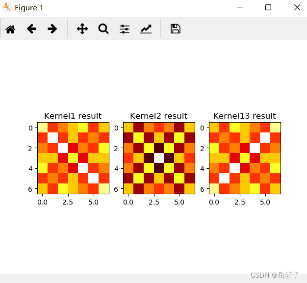
观察这三个特征图:
plt.figure()
plt.subplot(131).set_title('Kernel1 result')
plt.imshow(feature_map[0], cmap=plt.cm.hot, vmin=-1, vmax=1)
plt.subplot(132).set_title('Kernel2 result')
plt.imshow(feature_map[1], cmap=plt.cm.hot, vmin=-1, vmax=1)
plt.subplot(133).set_title('Kernel13 result')
plt.imshow(feature_map[2], cmap=plt.cm.hot, vmin=-1, vmax=1)
plt.show()
运行结果:
池化操作
池化过程 在通过卷积层获得特征(feature map) 之后 ,下一步要做的就是利用这些特征进行整合、分类。理论上来讲,所有经过卷积提取得到的特征都可以作为分类器的输入(比如 softmax 分类器) ,但这样做会面临着巨大的计算量. 比如对于一个 300X300 的输入图像(假设只有一个通道) ,经过 100个 3X3 大小的卷积核进行卷积操作后,得到的特征矩阵大小是 (300 -3+1) X(300 -3+1) = 88804 ,将这些数据一下输入到分类器中显然不好
此时我们就会采用 池化层将得到的特征(feature map) 进行降维,假如我们得到一个局部特征,他是一个图像的一个局部放大图,分辨率很大,那么我们就可以将一些像素点周围的像素点(特征值) 近似看待,将平面内某一位置及其相邻位置的特征值进行统计,并将汇总后的结果作为这一位置在该平面的值.
常见的池化有 最大池化(Max Pooling) , 平均池化(Average Pooling) ,使用池化函数来进一步对卷积操作得到的特征映射结果进行处理。池化会将平面内某未知及其相邻位置的特征值进行统计汇总。并将汇总后的结果作为这一位置在该平面的值。使用池化不会造成数据矩阵深度的改变,只会在高度和宽带上降低,达到降维的目的。
最大池化
最大池化会计算该位置及其相邻矩阵区域内的最大值,并将这个最大值作为该位置的值。

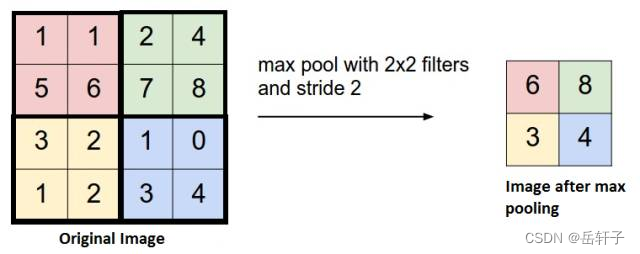
在我看来,其实就是在一个矩阵里面找出最大值。
因为这个矩阵的边长是奇数,咱们先补零,补成偶数。
补零操作:
pooling_stride = 2  # 步长
pooling_h = 4  # 特征图的高
pooling_w = 4  # 特征图的宽
feature_map_pad_0 = [[0 for i in range(0, 8)] for j in range(0, 8)]
for i in range(0, 3):  # 特征图 补0
    feature_map_pad_0[i] = np.pad(feature_map[i], ((0, 1), (0, 1)), 'constant', constant_values=(0, 0))

print("feature_map_pad_0 0:\n", np.around(feature_map_pad_0[0], decimals=2))
print("feature_map_pad_0 1:\n", np.around(feature_map_pad_0[1], decimals=2))
print("feature_map_pad_0 2:\n", np.around(feature_map_pad_0[2], decimals=2))
运行结果:
feature_map_pad_0 0:
 [[ 0.78 -0.11  0.11  0.33  0.56 -0.11  0.33  0.  ]
 [-0.11  1.   -0.11  0.33 -0.11  0.11 -0.11  0.  ]
 [ 0.11 -0.11  1.   -0.33  0.11 -0.11  0.56  0.  ]
 [ 0.33  0.33 -0.33  0.56 -0.33  0.33  0.33  0.  ]
 [ 0.56 -0.11  0.11 -0.33  1.   -0.11  0.11  0.  ]
 [-0.11  0.11 -0.11  0.33 -0.11  1.   -0.11  0.  ]
 [ 0.33 -0.11  0.56  0.33  0.11 -0.11  0.78  0.  ]
 [ 0.    0.    0.    0.    0.    0.    0.    0.  ]]
feature_map_pad_0 1:
 [[ 0.33 -0.56  0.11 -0.11  0.11 -0.56  0.33  0.  ]
 [-0.56  0.56 -0.56  0.33 -0.56  0.56 -0.56  0.  ]
 [ 0.11 -0.56  0.56 -0.78  0.56 -0.56  0.11  0.  ]
 [-0.11  0.33 -0.78  1.   -0.78  0.33 -0.11  0.  ]
 [ 0.11 -0.56  0.56 -0.78  0.56 -0.56  0.11  0.  ]
 [-0.56  0.56 -0.56  0.33 -0.56  0.56 -0.56  0.  ]
 [ 0.33 -0.56  0.11 -0.11  0.11 -0.56  0.33  0.  ]
 [ 0.    0.    0.    0.    0.    0.    0.    0.  ]]
feature_map_pad_0 2:
 [[ 0.33 -0.11  0.56  0.33  0.11 -0.11  0.78  0.  ]
 [-0.11  0.11 -0.11  0.33 -0.11  1.   -0.11  0.  ]
 [ 0.56 -0.11  0.11 -0.33  1.   -0.11  0.11  0.  ]
 [ 0.33  0.33 -0.33  0.56 -0.33  0.33  0.33  0.  ]
 [ 0.11 -0.11  1.   -0.33  0.11 -0.11  0.56  0.  ]
 [-0.11  1.   -0.11  0.33 -0.11  0.11 -0.11  0.  ]
 [ 0.78 -0.11  0.11  0.33  0.56 -0.11  0.33  0.  ]
 [ 0.    0.    0.    0.    0.    0.    0.    0.  ]]
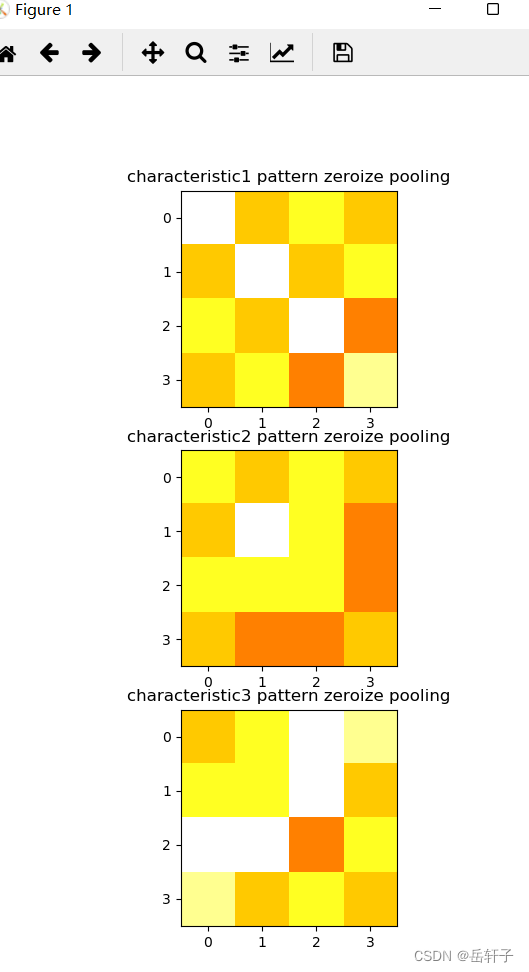
最大池化:
pooling = [0 for i in range(0, 3)]
for i in range(0, 3):
    pooling[i] = np.zeros((pooling_h, pooling_w))  # 初始化特征图
for h in range(pooling_h):  # 向下滑动,得到卷积后的固定行
    for w in range(pooling_w):  # 向右滑动,得到卷积后的固定行的列
        v_start = h * pooling_stride  # 滑动窗口的起始行(高)
        v_end = v_start + 2  # 滑动窗口的结束行(高)
        h_start = w * pooling_stride  # 滑动窗口的起始列(宽)
        h_end = h_start + 2  # 滑动窗口的结束列(宽)
        for i in range(0, 3):
            pooling[i][h, w] = np.max(feature_map_pad_0[i][v_start:v_end, h_start:h_end])

print("pooling:\n", np.around(pooling[0], decimals=2))
print("pooling:\n", np.around(pooling[1], decimals=2))
print("pooling:\n", np.around(pooling[2], decimals=2))

plt.figure()
plt.subplot(311).set_title('characteristic1 pattern zeroize pooling')
plt.imshow(pooling[0], cmap=plt.cm.hot, vmin=-1, vmax=1)
plt.subplot(312).set_title('characteristic2 pattern zeroize pooling')
plt.imshow(pooling[1], cmap=plt.cm.hot, vmin=-1, vmax=1)
plt.subplot(313).set_title('characteristic3 pattern zeroize pooling')
plt.imshow(pooling[2], cmap=plt.cm.hot, vmin=-1, vmax=1)
plt.show()
运行结果:
pooling:
 [[1.   0.33 0.56 0.33]
 [0.33 1.   0.33 0.56]
 [0.56 0.33 1.   0.11]
 [0.33 0.56 0.11 0.78]]
pooling:
 [[0.56 0.33 0.56 0.33]
 [0.33 1.   0.56 0.11]
 [0.56 0.56 0.56 0.11]
 [0.33 0.11 0.11 0.33]]
pooling:
 [[0.33 0.56 1.   0.78]
 [0.56 0.56 1.   0.33]
 [1.   1.   0.11 0.56]
 [0.78 0.33 0.56 0.33]]
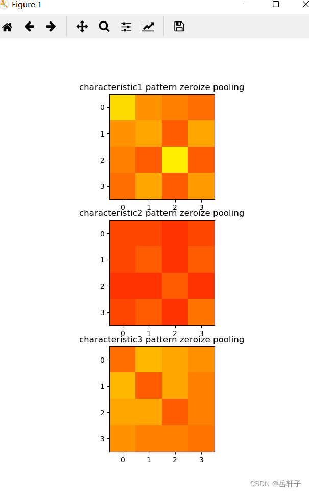
平均池化
平均池化会计算该位置及其相邻矩阵区域内的平均值,并将这个值作为该位置的值。
相对于最大池化,平均池化就是求一个矩阵的平均值
pooling = [0 for i in range(0, 3)]
for i in range(0, 3):
    pooling[i] = np.zeros((pooling_h, pooling_w))  # 初始化特征图
for h in range(pooling_h):  # 向下滑动,得到卷积后的固定行
    for w in range(pooling_w):  # 向右滑动,得到卷积后的固定行的列
        v_start = h * pooling_stride  # 滑动窗口的起始行(高)
        v_end = v_start + 2  # 滑动窗口的结束行(高)
        h_start = w * pooling_stride  # 滑动窗口的起始列(宽)
        h_end = h_start + 2  # 滑动窗口的结束列(宽)
        for i in range(0, 3):
            pooling[i][h, w] = np.mean(feature_map_pad_0[i][v_start:v_end, h_start:h_end])

print("pooling:\n", np.around(pooling[0], decimals=2))
print("pooling:\n", np.around(pooling[1], decimals=2))
print("pooling:\n", np.around(pooling[2], decimals=2))

plt.figure()
plt.subplot(311).set_title('characteristic1 pattern zeroize pooling')
plt.imshow(pooling[0], cmap=plt.cm.hot, vmin=-1, vmax=1)
plt.subplot(312).set_title('characteristic2 pattern zeroize pooling')
plt.imshow(pooling[1], cmap=plt.cm.hot, vmin=-1, vmax=1)
plt.subplot(313).set_title('characteristic3 pattern zeroize pooling')
plt.imshow(pooling[2], cmap=plt.cm.hot, vmin=-1, vmax=1)
plt.show()
运行结果:
pooling:
 [[0.39 0.17 0.11 0.06]
 [0.17 0.22 0.   0.22]
 [0.11 0.   0.44 0.  ]
 [0.06 0.22 0.   0.19]]
pooling:
 [[-0.06 -0.06 -0.11 -0.06]
 [-0.06  0.   -0.11  0.  ]
 [-0.11 -0.11  0.   -0.11]
 [-0.06  0.   -0.11  0.08]]
pooling:
 [[0.06 0.28 0.22 0.17]
 [0.28 0.   0.22 0.11]
 [0.22 0.22 0.   0.11]
 [0.17 0.11 0.11 0.08]]
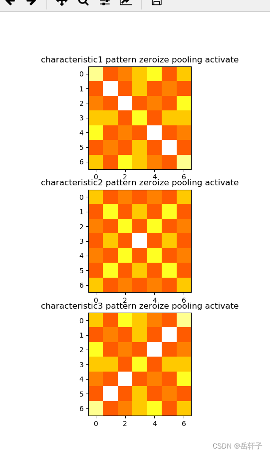
激活操作
这里我们用relu函数(这里衔接的上面的平均池化)
# 激活
# 激活函数
def relu(x):
    return (abs(x) + x) / 2

relu_map_h = 7  # 特征图的高
relu_map_w = 7  # 特征图的宽
relu_map = [0 for i in range(0, 3)]  # 初始化3个特征图
for i in range(0, 3):
    relu_map[i] = np.zeros((relu_map_h, relu_map_w))  # 初始化特征图

for i in range(0, 3):
    relu_map[i] = relu(feature_map[i])

print("relu map :\n", np.around(relu_map[0], decimals=2))
print("relu map :\n", np.around(relu_map[1], decimals=2))
print("relu map :\n", np.around(relu_map[2], decimals=2))
plt.figure()
plt.subplot(311).set_title('characteristic1 pattern zeroize pooling activate')
plt.imshow(relu_map[0], cmap=plt.cm.hot, vmin=-1, vmax=1)
plt.subplot(312).set_title('characteristic2 pattern zeroize pooling activate')
plt.imshow(relu_map[1], cmap=plt.cm.hot, vmin=-1, vmax=1)
plt.subplot(313).set_title('characteristic3 pattern zeroize pooling activate')
plt.imshow(relu_map[2], cmap=plt.cm.hot, vmin=-1, vmax=1)
plt.show()
运行结果:
relu map :
 [[0.33 0.   0.56 0.33 0.11 0.   0.78]
 [0.   0.11 0.   0.33 0.   1.   0.  ]
 [0.56 0.   0.11 0.   1.   0.   0.11]
 [0.33 0.33 0.   0.56 0.   0.33 0.33]
 [0.11 0.   1.   0.   0.11 0.   0.56]
 [0.   1.   0.   0.33 0.   0.11 0.  ]
 [0.78 0.   0.11 0.33 0.56 0.   0.33]]
2、pytorch版本(利用pytorch框架)
2.1相关函数
这里用pytorch来实现卷积的话,会方便很多。有很多卷积计算的函数。
- torch.nn.Conv2d(in_channels, out_channels, kernel_size, stride=1, padding=0, dilation=1, groups=1, bias=True)
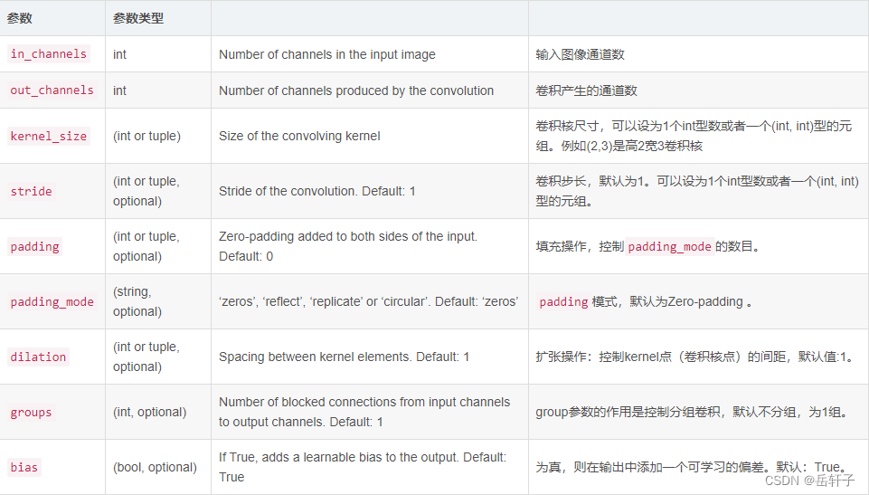
- torch.nn.MaxPool2d(kernel_size,stride,padding,dilation,return_indices,ceil_mode)
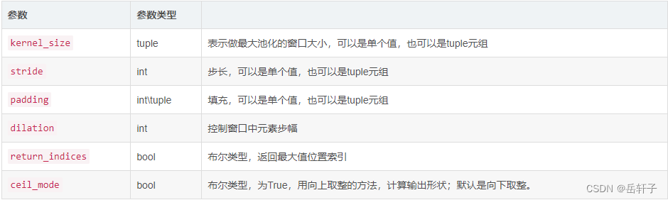
- torch.nn.ZeroPad2d()

2.1图像
代码:
import torch
import torch.nn as nn
import matplotlib.pyplot as plt

pic = torch.tensor([[[[-1, -1, -1, -1, -1, -1, -1, -1, -1],
                    [-1, 1, -1, -1, -1, -1, -1, 1, -1],
                    [-1, -1, 1, -1, -1, -1, 1, -1, -1],
                    [-1, -1, -1, 1, -1, 1, -1, -1, -1],
                    [-1, -1, -1, -1, 1, -1, -1, -1, -1],
                    [-1, -1, -1, 1, -1, 1, -1, -1, -1],
                    [-1, -1, 1, -1, -1, -1, 1, -1, -1],
                    [-1, 1, -1, -1, -1, -1, -1, 1, -1],
                    [-1, -1, -1, -1, -1, -1, -1, -1, -1]]]], dtype=torch.float)
img = pic.data.squeeze().numpy()  # 将输出转换为图片的格式
2.2 卷积核
conv1 = nn.Conv2d(1, 1, (3, 3), 1)  # in_channel , out_channel , kennel_size , stride
conv1.weight.data = torch.Tensor([[[[1, -1, -1],
                                    [-1, 1, -1],
                                    [-1, -1, 1]]
                                   ]])
img2 = conv1.weight.data.squeeze().numpy()  # 将输出转换为图片的格式
conv2 = nn.Conv2d(1, 1, (3, 3), 1)  # in_channel , out_channel , kennel_size , stride
conv2.weight.data = torch.Tensor([[[[1, -1, 1],
                                    [-1, 1, -1],
                                    [1, -1, 1]]
                                   ]])
img3 = conv2.weight.data.squeeze().numpy()  # 将输出转换为图片的格式
conv3 = nn.Conv2d(1, 1, (3, 3), 1)  # in_channel , out_channel , kennel_size , stride
conv3.weight.data = torch.Tensor([[[[-1, -1, 1],
                                    [-1, 1, -1],
                                    [1, -1, -1]]
                                   ]])
img4 = conv3.weight.data.squeeze().numpy()  # 将输出转换为图片的格式
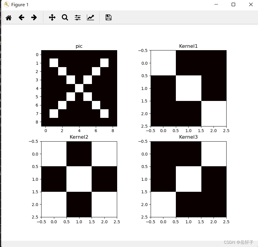
观察图像:
plt.subplot(221).set_title('pic')
plt.imshow(img, cmap=plt.cm.hot, vmin=-1, vmax=1)
plt.subplot(222).set_title('Kernel1')
plt.imshow(img2, cmap=plt.cm.hot, vmin=-1, vmax=1)
plt.subplot(223).set_title('Kernel2')
plt.imshow(img3, cmap=plt.cm.hot, vmin=-1, vmax=1)
plt.subplot(224).set_title('Kernel3')
plt.imshow(img4, cmap=plt.cm.hot, vmin=-1, vmax=1)
plt.show()
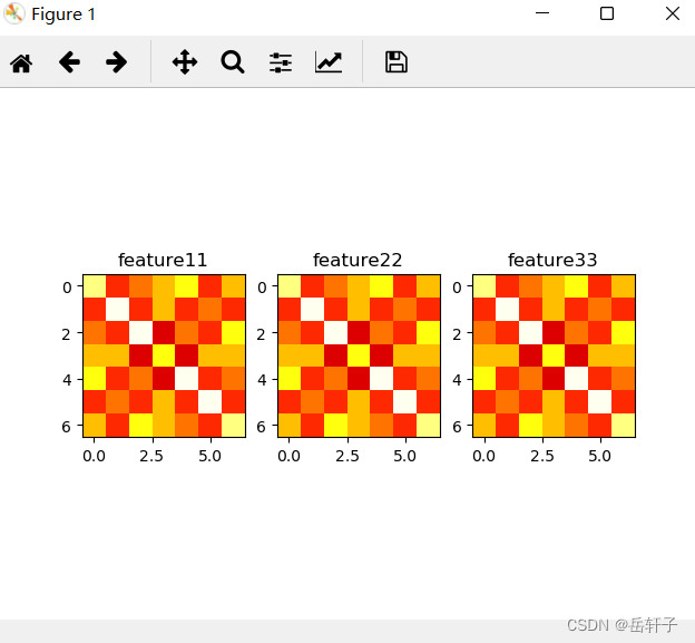
2.3 进行卷积操作
# 进行卷积操作
feature_map1 = conv1(pic) / 9
feature_map2 = conv2(pic) / 9
feature_map3 = conv3(pic) / 9

print(feature_map1 / 9)
print(feature_map2 / 9)
print(feature_map3 / 9)
feature_map11 = feature_map1.data.squeeze().numpy()  # 将输出转换为图片的格式
feature_map22 = feature_map1.data.squeeze().numpy()  # 将输出转换为图片的格式
feature_map33 = feature_map1.data.squeeze().numpy()  # 将输出转换为图片的格式

plt.subplot(131).set_title('feature1')
plt.imshow(feature_map11, cmap=plt.cm.hot, vmin=-1, vmax=1)
plt.subplot(132).set_title('feature2')
plt.imshow(feature_map22, cmap=plt.cm.hot, vmin=-1, vmax=1)
plt.subplot(133).set_title('feature3')
plt.imshow(feature_map33, cmap=plt.cm.hot, vmin=-1, vmax=1)
plt.show()
运行结果:
tensor([[[[ 0.0826, -0.0162,  0.0085,  0.0332,  0.0579, -0.0162,  0.0332],
          [-0.0162,  0.1073, -0.0162,  0.0332, -0.0162,  0.0085, -0.0162],
          [ 0.0085, -0.0162,  0.1073, -0.0409,  0.0085, -0.0162,  0.0579],
          [ 0.0332,  0.0332, -0.0409,  0.0579, -0.0409,  0.0332,  0.0332],
          [ 0.0579, -0.0162,  0.0085, -0.0409,  0.1073, -0.0162,  0.0085],
          [-0.0162,  0.0085, -0.0162,  0.0332, -0.0162,  0.1073, -0.0162],
          [ 0.0332, -0.0162,  0.0579,  0.0332,  0.0085, -0.0162,  0.0826]]]],
       grad_fn=<DivBackward0>)
tensor([[[[ 0.0401, -0.0586,  0.0155, -0.0092,  0.0155, -0.0586,  0.0401],
          [-0.0586,  0.0648, -0.0586,  0.0401, -0.0586,  0.0648, -0.0586],
          [ 0.0155, -0.0586,  0.0648, -0.0833,  0.0648, -0.0586,  0.0155],
          [-0.0092,  0.0401, -0.0833,  0.1142, -0.0833,  0.0401, -0.0092],
          [ 0.0155, -0.0586,  0.0648, -0.0833,  0.0648, -0.0586,  0.0155],
          [-0.0586,  0.0648, -0.0586,  0.0401, -0.0586,  0.0648, -0.0586],
          [ 0.0401, -0.0586,  0.0155, -0.0092,  0.0155, -0.0586,  0.0401]]]],
       grad_fn=<DivBackward0>)
tensor([[[[ 0.0395, -0.0099,  0.0642,  0.0395,  0.0148, -0.0099,  0.0889],
          [-0.0099,  0.0148, -0.0099,  0.0395, -0.0099,  0.1136, -0.0099],
          [ 0.0642, -0.0099,  0.0148, -0.0346,  0.1136, -0.0099,  0.0148],
          [ 0.0395,  0.0395, -0.0346,  0.0642, -0.0346,  0.0395,  0.0395],
          [ 0.0148, -0.0099,  0.1136, -0.0346,  0.0148, -0.0099,  0.0642],
          [-0.0099,  0.1136, -0.0099,  0.0395, -0.0099,  0.0148, -0.0099],
          [ 0.0889, -0.0099,  0.0148,  0.0395,  0.0642, -0.0099,  0.0395]]]],
       grad_fn=<DivBackward0>)
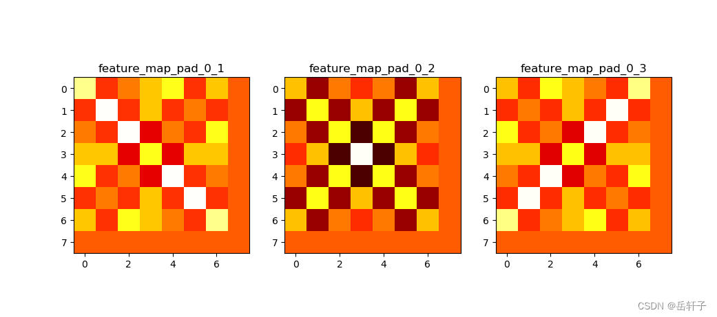
2.4 进行池化
最大池化与平均池化
代码:
max_pool = nn.MaxPool2d(2, padding=0, stride=2) # Pooling
mean_pool = nn.AvgPool2d(2, padding=0, stride=2) # Pooling
zeroPad = nn.ZeroPad2d(padding=(0, 1, 0, 1)) # pad 0 , Left Right Up Down
# 最大池化
feature_map_pad_0_1 = zeroPad(feature_map1)
feature_pool_1 = max_pool(feature_map_pad_0_1)
feature_map_pad_0_2 = zeroPad(feature_map2)
feature_pool_2 = max_pool(feature_map_pad_0_2)
feature_map_pad_0_3 = zeroPad(feature_map3)
feature_pool_3 = max_pool(feature_map_pad_0_3)
# 平均池化
feature_map_pad_0_1 = zeroPad(feature_map1)
feature_mean_pool_1 = mean_pool(feature_map_pad_0_1)
feature_map_pad_0_2 = zeroPad(feature_map2)
feature_mean_pool_2 = mean_pool(feature_map_pad_0_2)
feature_map_pad_0_3 = zeroPad(feature_map3)
feature_mean_pool_3 = mean_pool(feature_map_pad_0_3)
print(feature_pool_1.size())
print(feature_pool_1 / 9)
print(feature_pool_2 / 9)
print(feature_pool_3 / 9)
img = feature_pool_1.data.squeeze().numpy() # 将输出转换为图片的格式
plt.subplot(131).set_title('feature_map_pad_0_1')
plt.imshow(feature_map_pad_0_1.data.squeeze().numpy(), cmap=plt.cm.hot, vmin=-1, vmax=1)
plt.subplot(132).set_title('feature_map_pad_0_2')
plt.imshow(feature_map_pad_0_2.data.squeeze().numpy(), cmap=plt.cm.hot, vmin=-1, vmax=1)
plt.subplot(133).set_title('feature_map_pad_0_3')
plt.imshow(feature_map_pad_0_3.data.squeeze().numpy(), cmap=plt.cm.hot, vmin=-1, vmax=1)
plt.show()
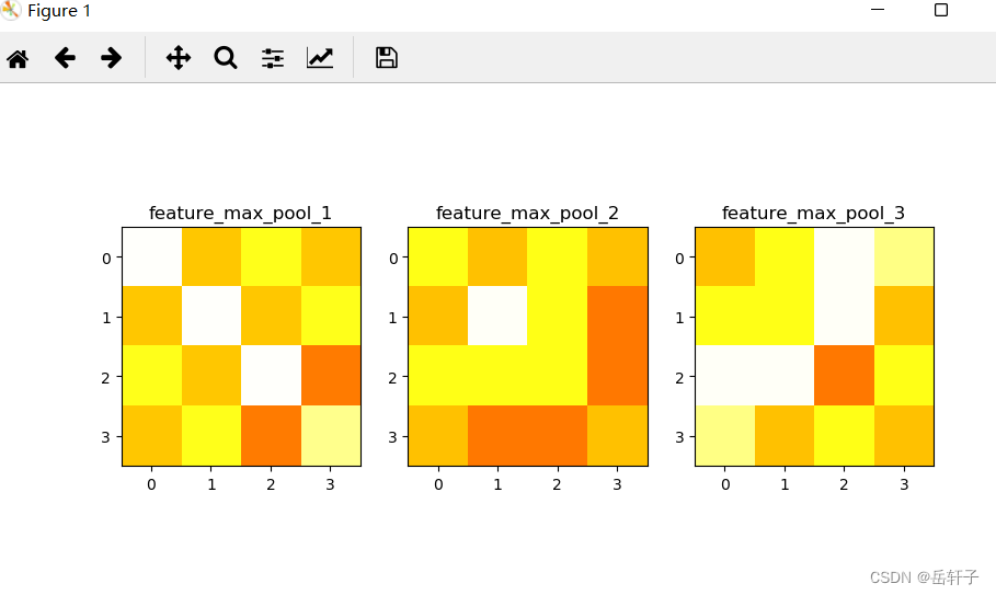
plt.subplot(131).set_title('feature_max_pool_1')
plt.imshow(feature_pool_1.data.squeeze().numpy(), cmap=plt.cm.hot, vmin=-1, vmax=1)
plt.subplot(132).set_title('feature_max_pool_2')
plt.imshow(feature_pool_2.data.squeeze().numpy(), cmap=plt.cm.hot, vmin=-1, vmax=1)
plt.subplot(133).set_title('feature_max_pool_3')
plt.imshow(feature_pool_3.data.squeeze().numpy(), cmap=plt.cm.hot, vmin=-1, vmax=1)
plt.show()
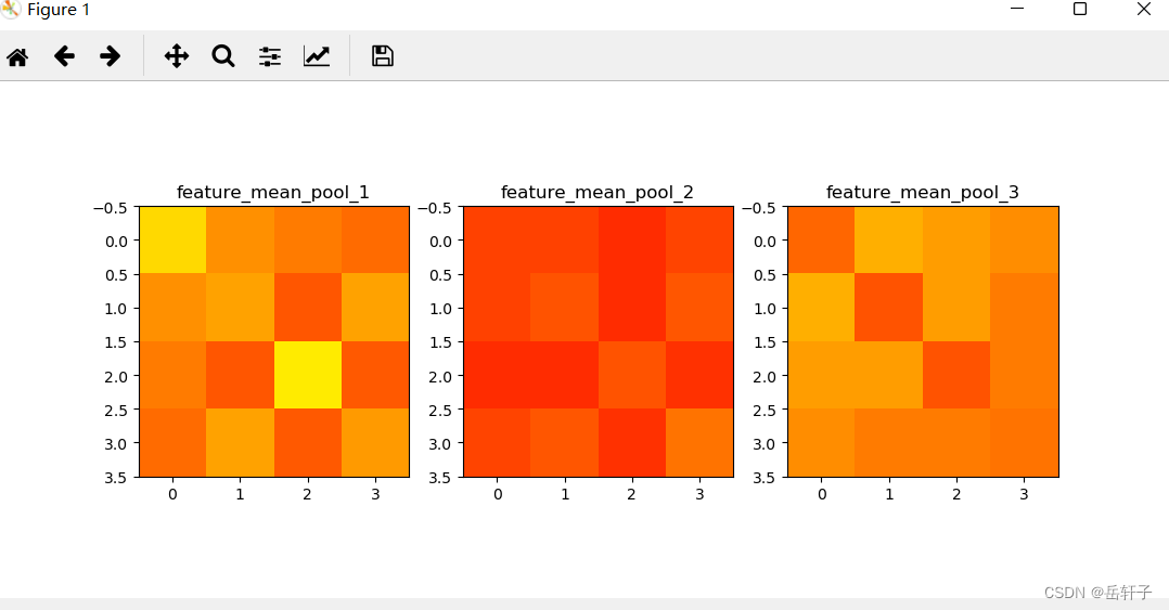
plt.subplot(131).set_title('feature_mean_pool_1')
plt.imshow(feature_mean_pool_1.data.squeeze().numpy(), cmap=plt.cm.hot, vmin=-1, vmax=1)
plt.subplot(132).set_title('feature_mean_pool_2')
plt.imshow(feature_mean_pool_2.data.squeeze().numpy(), cmap=plt.cm.hot, vmin=-1, vmax=1)
plt.subplot(133).set_title('feature_mean_pool_3')
plt.imshow(feature_mean_pool_3.data.squeeze().numpy(), cmap=plt.cm.hot, vmin=-1, vmax=1)
plt.show()
运行结果:
torch.Size([1, 1, 4, 4])
tensor([[[[0.1100, 0.0360, 0.0607, 0.0360],
          [0.0360, 0.1100, 0.0360, 0.0607],
          [0.0607, 0.0360, 0.1100, 0.0113],
          [0.0360, 0.0607, 0.0113, 0.0853]]]], grad_fn=<DivBackward0>)
tensor([[[[0.0593, 0.0346, 0.0593, 0.0346],
          [0.0346, 0.1087, 0.0593, 0.0099],
          [0.0593, 0.0593, 0.0593, 0.0099],
          [0.0346, 0.0099, 0.0099, 0.0346]]]], grad_fn=<DivBackward0>)
tensor([[[[0.0344, 0.0591, 0.1085, 0.0838],
          [0.0591, 0.0591, 0.1085, 0.0344],
          [0.1085, 0.1085, 0.0098, 0.0591],
          [0.0838, 0.0344, 0.0591, 0.0344]]]], grad_fn=<DivBackward0>)
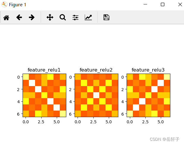
2.5 激活函数进行激活
对卷积图像进行激活
activation_function = nn.ReLU()
feature_relu1 = activation_function(feature_map1)
feature_relu2 = activation_function(feature_map2)
feature_relu3 = activation_function(feature_map3)
print(feature_relu1 / 9)
print(feature_relu2 / 9)
print(feature_relu3 / 9)
plt.subplot(131).set_title('feature_relu1')
plt.imshow(feature_relu1.data.squeeze().numpy(), cmap=plt.cm.hot, vmin=-1, vmax=1)
plt.subplot(132).set_title('feature_relu2')
plt.imshow(feature_relu2.data.squeeze().numpy(), cmap=plt.cm.hot, vmin=-1, vmax=1)
plt.subplot(133).set_title('feature_relu3')
plt.imshow(feature_relu3.data.squeeze().numpy(), cmap=plt.cm.hot, vmin=-1, vmax=1)
plt.show()
运行结果:
tensor([[[[0.0832, 0.0000, 0.0091, 0.0338, 0.0585, 0.0000, 0.0338],
          [0.0000, 0.1079, 0.0000, 0.0338, 0.0000, 0.0091, 0.0000],
          [0.0091, 0.0000, 0.1079, 0.0000, 0.0091, 0.0000, 0.0585],
          [0.0338, 0.0338, 0.0000, 0.0585, 0.0000, 0.0338, 0.0338],
          [0.0585, 0.0000, 0.0091, 0.0000, 0.1079, 0.0000, 0.0091],
          [0.0000, 0.0091, 0.0000, 0.0338, 0.0000, 0.1079, 0.0000],
          [0.0338, 0.0000, 0.0585, 0.0338, 0.0091, 0.0000, 0.0832]]]],
       grad_fn=<DivBackward0>)
tensor([[[[0.0332, 0.0000, 0.0085, 0.0000, 0.0085, 0.0000, 0.0332],
          [0.0000, 0.0579, 0.0000, 0.0332, 0.0000, 0.0579, 0.0000],
          [0.0085, 0.0000, 0.0579, 0.0000, 0.0579, 0.0000, 0.0085],
          [0.0000, 0.0332, 0.0000, 0.1073, 0.0000, 0.0332, 0.0000],
          [0.0085, 0.0000, 0.0579, 0.0000, 0.0579, 0.0000, 0.0085],
          [0.0000, 0.0579, 0.0000, 0.0332, 0.0000, 0.0579, 0.0000],
          [0.0332, 0.0000, 0.0085, 0.0000, 0.0085, 0.0000, 0.0332]]]],
       grad_fn=<DivBackward0>)
tensor([[[[0.0378, 0.0000, 0.0625, 0.0378, 0.0131, 0.0000, 0.0872],
          [0.0000, 0.0131, 0.0000, 0.0378, 0.0000, 0.1119, 0.0000],
          [0.0625, 0.0000, 0.0131, 0.0000, 0.1119, 0.0000, 0.0131],
          [0.0378, 0.0378, 0.0000, 0.0625, 0.0000, 0.0378, 0.0378],
          [0.0131, 0.0000, 0.1119, 0.0000, 0.0131, 0.0000, 0.0625],
          [0.0000, 0.1119, 0.0000, 0.0378, 0.0000, 0.0131, 0.0000],
          [0.0872, 0.0000, 0.0131, 0.0378, 0.0625, 0.0000, 0.0378]]]],
       grad_fn=<DivBackward0>)
二、基于CNN的XO识别
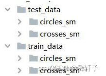
1、数据集准备
XO数据集:
文件夹train_data:放置训练集 1700张图片,为850张X和850张O
文件夹test_data: 放置测试集 300张图片,为150张X和150张O
这个文件夹是自己设置的
导入数据:
import torch
from torchvision import transforms, datasets
import torch.nn as nn
from torch.utils.data import DataLoader
import torch.optim as optim
import matplotlib.pyplot as plt


transforms = transforms.Compose([
    transforms.ToTensor(),  # 把图片进行归一化,并把数据转换成Tensor类型
    transforms.Grayscale(1)  # 把图片 转为灰度图
])

path_test = r'E:\桌面资料\机器学习实验\复习\dataXO\test_data'
path = r'E:\桌面资料\机器学习实验\复习\dataXO\train_data'

data_train = datasets.ImageFolder(path, transform=transforms)
data_test = datasets.ImageFolder(path_test, transform=transforms)

print("size of train_data:", len(data_train))
print("size of test_data:", len(data_test))

data_loader = DataLoader(data_train, batch_size=64, shuffle=True)
data_loader_test = DataLoader(data_test, batch_size=64, shuffle=True)

for i, data in enumerate(data_loader):
    images, labels = data
    print(images.shape)
    print(labels.shape)
    break

for i, data in enumerate(data_loader_test):
    images, labels = data
    print(images.shape)
    print(labels.shape)
    break
运行结果:
size of train_data: 1700
size of test_data: 300
torch.Size([64, 1, 116, 116])
torch.Size([64])
torch.Size([64, 1, 116, 116])
torch.Size([64])
2、 构建模型
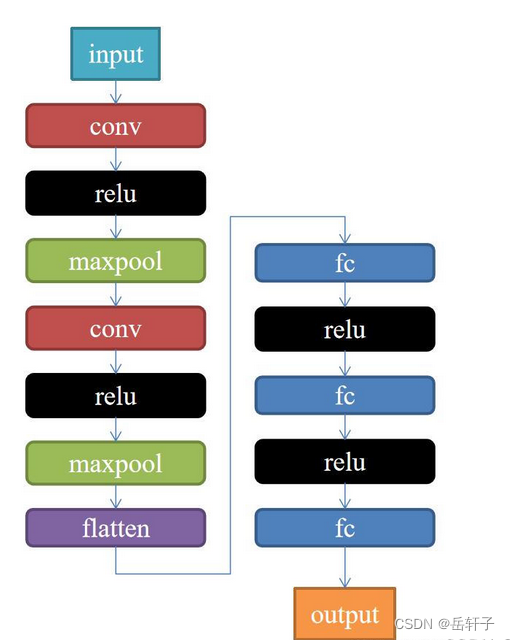
class Net(nn.Module):
    def __init__(self):
        super(Net, self).__init__()
        self.conv1 = nn.Conv2d(1, 9, 3)
        self.maxpool = nn.MaxPool2d(2, 2)
        self.conv2 = nn.Conv2d(9, 5, 3)

        self.relu = nn.ReLU()
        self.fc1 = nn.Linear(27 * 27 * 5, 1200)
        self.fc2 = nn.Linear(1200, 64)
        self.fc3 = nn.Linear(64, 2)

    def forward(self, x):
        x = self.maxpool(self.relu(self.conv1(x)))
        x = self.maxpool(self.relu(self.conv2(x)))
        x = x.view(-1, 27 * 27 * 5)
        x = self.relu(self.fc1(x))
        x = self.relu(self.fc2(x))
        x = self.fc3(x)
        return x
3、训练模型
model = Net()

criterion = torch.nn.CrossEntropyLoss()  # 损失函数 交叉熵损失函数
optimizer = optim.SGD(model.parameters(), lr=0.1)  # 优化函数:随机梯度下降

epochs = 10
for epoch in range(epochs):
    running_loss = 0.0
    for i, data in enumerate(data_loader):
        images, label = data
        out = model(images)
        loss = criterion(out, label)

        optimizer.zero_grad()
        loss.backward()
        optimizer.step()

        running_loss += loss.item()
        if (i + 1) % 10 == 0:
            print('[%d  %5d]   loss: %.3f' % (epoch + 1, i + 1, running_loss / 100))
            running_loss = 0.0

print('finished train')

# 保存模型
torch.save(model, 'model_name.pth')  # 保存的是模型, 不止是w和b权重值
运行结果:
[1     10]   loss: 0.069
[1     20]   loss: 0.069
[2     10]   loss: 0.069
[2     20]   loss: 0.068
[3     10]   loss: 0.066
[3     20]   loss: 0.058
[4     10]   loss: 0.079
[4     20]   loss: 0.070
[6     20]   loss: 0.070
[7     10]   loss: 0.069
[7     20]   loss: 0.065
[8     10]   loss: 0.023
[8     20]   loss: 0.030
[9     10]   loss: 0.365
[9     20]   loss: 0.070
[10     10]   loss: 0.070
[10     20]   loss: 0.069
finished train
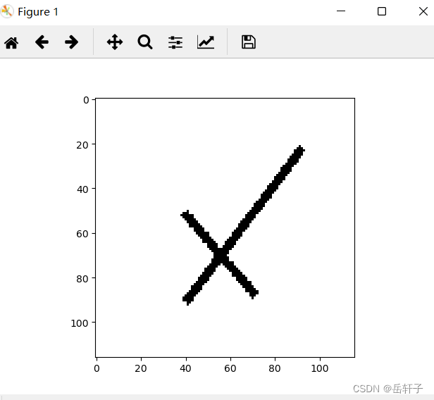
4、测试训练好的模型
# 读取模型
model_load = torch.load('model_name.pth')
# 读取一张图片 images[0],测试
print("labels[0] truth:\t", labels[0])
x = images[0]
x = x.reshape([1, x.shape[0], x.shape[1], x.shape[2]])
predicted = torch.max(model_load(x), 1)
print("labels[0] predict:\t", predicted.indices)

img = images[0].data.squeeze().numpy()  # 将输出转换为图片的格式
plt.imshow(img, cmap='gray')
plt.show()
运行结果:
labels[0] truth:         tensor(0)
labels[0] predict:       tensor([1])
5、计算模型的准确率
# 读取模型
model_load = torch.load('model_name.pth')

correct = 0
total = 0
with torch.no_grad():  # 进行评测的时候网络不更新梯度
    for data in data_loader_test:  # 读取测试集
        images, labels = data
        outputs = model_load(images)
        _, predicted = torch.max(outputs.data, 1)  # 取出 最大值的索引 作为 分类结果
        total += labels.size(0)  # labels 的长度
        correct += (predicted == labels).sum().item()  # 预测正确的数目
print('Accuracy of the network on the  test images: %f %%' % (100. * correct / total))
运行结果:
Accuracy of the network on the test images: 99.333333 %
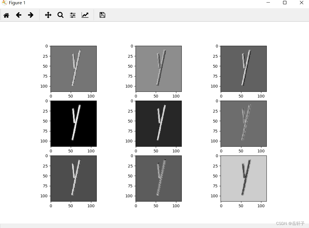
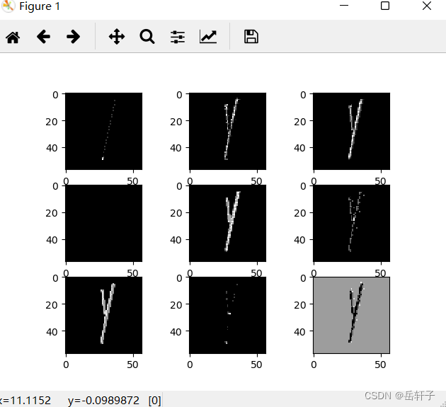
6、查看训练好的模型特征图
import torch
import matplotlib.pyplot as plt
import numpy as np
from torchvision import transforms, datasets
import torch.nn as nn
from torch.utils.data import DataLoader

# 定义图像预处理过程
transforms = transforms.Compose([
    transforms.ToTensor(),  # 把图片进行归一化,并把数据转换成Tensor类型
    transforms.Grayscale(1)  # 把图片 转为灰度图
])
path = r'路径'
data_train = datasets.ImageFolder(path, transform=transforms)
data_loader = DataLoader(data_train, batch_size=64, shuffle=True)
for i, data in enumerate(data_loader):
    images, labels = data
    print(images.shape)
    print(labels.shape)
    break


class Net(nn.Module):
    def __init__(self):
        super(Net, self).__init__()
        self.conv1 = nn.Conv2d(1, 9, 3)  # in_channel , out_channel , kennel_size , stride
        self.maxpool = nn.MaxPool2d(2, 2)
        self.conv2 = nn.Conv2d(9, 5, 3)  # in_channel , out_channel , kennel_size , stride

        self.relu = nn.ReLU()
        self.fc1 = nn.Linear(27 * 27 * 5, 1200)  # full connect 1
        self.fc2 = nn.Linear(1200, 64)  # full connect 2
        self.fc3 = nn.Linear(64, 2)  # full connect 3

    def forward(self, x):
        outputs = []
        x = self.conv1(x)
        outputs.append(x)
        x = self.relu(x)
        outputs.append(x)
        x = self.maxpool(x)
        outputs.append(x)
        x = self.conv2(x)
        x = self.relu(x)
        x = self.maxpool(x)
        x = x.view(-1, 27 * 27 * 5)
        x = self.relu(self.fc1(x))
        x = self.relu(self.fc2(x))
        x = self.fc3(x)
        return outputs

# load model weights加载预训练权重
model_weight_path = "model_name.pth"
model1 = torch.load(model_weight_path)

# 打印出模型的结构
print(model1)
x = images[0]
x = x.reshape([1, x.shape[0], x.shape[1], x.shape[2]])
# forward正向传播过程
out_put = model1(x)
for feature_map in out_put:
    im = np.squeeze(feature_map.detach().numpy())
    im = np.transpose(im, [1, 2, 0])
    print(im.shape)

    plt.figure()
    for i in range(9):
        ax = plt.subplot(3, 3, i + 1)
        plt.imshow(im[:, :, i], cmap='gray')
    plt.show()
运行结果:
torch.Size([64, 1, 116, 116])
torch.Size([64])
Net(
  (conv1): Conv2d(1, 9, kernel_size=(3, 3), stride=(1, 1))
  (maxpool): MaxPool2d(kernel_size=2, stride=2, padding=0, dilation=1, ceil_mode=False)
  (conv2): Conv2d(9, 5, kernel_size=(3, 3), stride=(1, 1))
  (relu): ReLU()
  (fc1): Linear(in_features=3645, out_features=1200, bias=True)
  (fc2): Linear(in_features=1200, out_features=64, bias=True)
  (fc3): Linear(in_features=64, out_features=2, bias=True)
)
(114, 114, 9)
(114, 114, 9)
(57, 57, 9)
第一轮的:
第二轮的
第三轮的
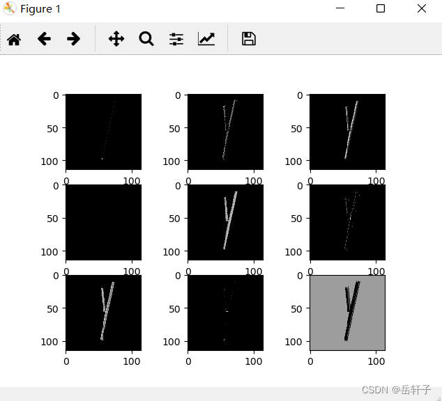
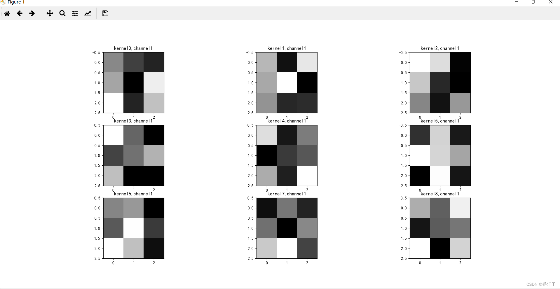
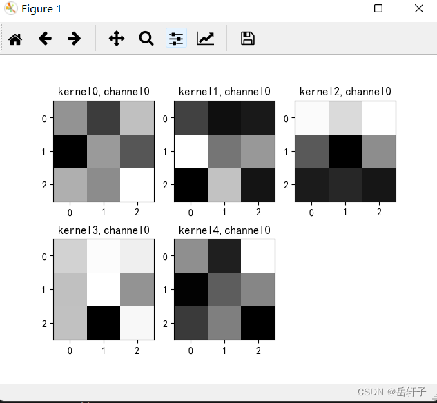
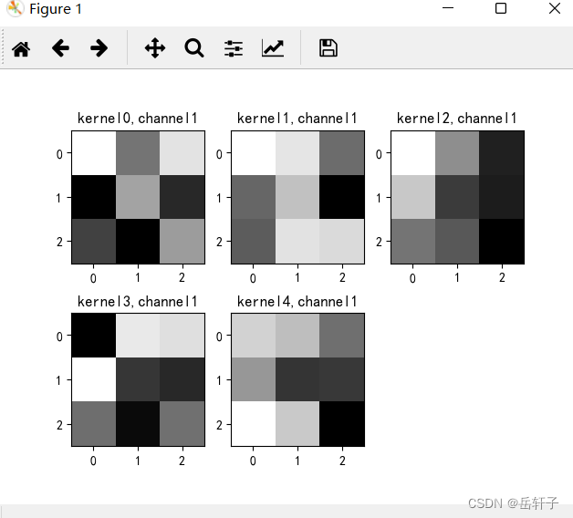
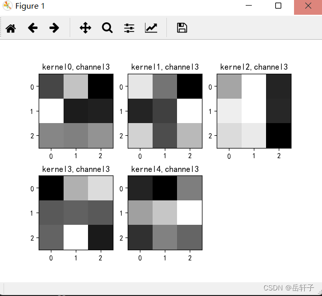
7、查看训练好的卷积核
import torch
import matplotlib.pyplot as plt
import numpy as np
from PIL import Image
from torchvision import transforms, datasets
import torch.nn as nn
from torch.utils.data import DataLoader
plt.rcParams['font.sans-serif'] = ['SimHei'] # 用来正常显示中文标签
plt.rcParams['axes.unicode_minus'] = False # 用来正常显示负号 #有中文出现的情况,需要u'内容
# 定义图像预处理过程(要与网络模型训练过程中的预处理过程一致)
transforms = transforms.Compose([
transforms.ToTensor(), # 把图片进行归一化,并把数据转换成Tensor类型
transforms.Grayscale(1) # 把图片 转为灰度图
])
path = r'D:\project\DL\training_data_sm'
data_train = datasets.ImageFolder(path, transform=transforms)
data_loader = DataLoader(data_train, batch_size=64, shuffle=True)
for i, data in enumerate(data_loader):
images, labels = data
break
class Net(nn.Module):
def __init__(self):
super(Net, self).__init__()
self.conv1 = nn.Conv2d(1, 9, 3) # in_channel , out_channel , kennel_size , stride
self.maxpool = nn.MaxPool2d(2, 2)
self.conv2 = nn.Conv2d(9, 5, 3) # in_channel , out_channel , kennel_size , stride
self.relu = nn.ReLU()
self.fc1 = nn.Linear(27 * 27 * 5, 1200) # full connect 1
self.fc2 = nn.Linear(1200, 64) # full connect 2
self.fc3 = nn.Linear(64, 2) # full connect 3
def forward(self, x):
outputs = []
x = self.maxpool(self.relu(self.conv1(x)))
# outputs.append(x)
x = self.maxpool(self.relu(self.conv2(x)))
outputs.append(x)
x = x.view(-1, 27 * 27 * 5)
x = self.relu(self.fc1(x))
x = self.relu(self.fc2(x))
x = self.fc3(x)
return outputs
# create model
model1 = Net()
# load model weights加载预训练权重
model_weight_path = "model_name1.pth"
model1.load_state_dict(torch.load(model_weight_path))
x = images[0]
x = x.reshape([1, x.shape[0], x.shape[1], x.shape[2]])
# forward正向传播过程
out_put = model1(x)
weights_keys = model1.state_dict().keys()
for key in weights_keys:
print("key :", key)
# 卷积核通道排列顺序 [kernel_number, kernel_channel, kernel_height, kernel_width]
if key == "conv1.weight":
weight_t = model1.state_dict()[key].numpy()
print("weight_t.shape", weight_t.shape)
k = weight_t[:, 0, :, :] # 获取第一个卷积核的信息参数
# show 9 kernel ,1 channel
plt.figure()
for i in range(9):
ax = plt.subplot(3, 3, i + 1) # 参数意义:3:图片绘制行数,5:绘制图片列数,i+1:图的索引
plt.imshow(k[i, :, :], cmap='gray')
title_name = 'kernel' + str(i) + ',channel1'
plt.title(title_name)
plt.show()
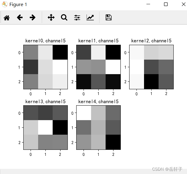
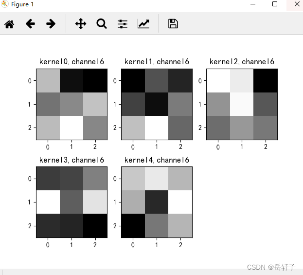
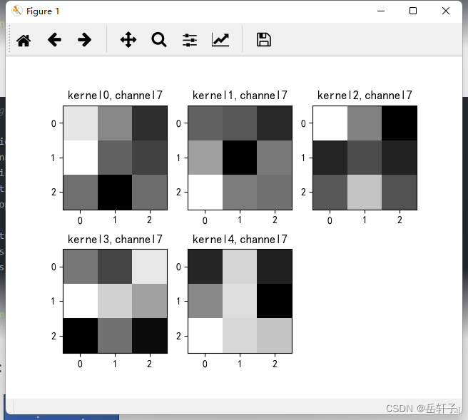
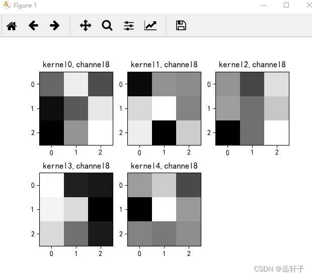
if key == "conv2.weight":
weight_t = model1.state_dict()[key].numpy()
print("weight_t.shape", weight_t.shape)
k = weight_t[:, :, :, :] # 获取第一个卷积核的信息参数
print(k.shape)
print(k)
plt.figure()
for c in range(9):
channel = k[:, c, :, :]
for i in range(5):
ax = plt.subplot(2, 3, i + 1) # 参数意义:3:图片绘制行数,5:绘制图片列数,i+1:图的索引
plt.imshow(channel[i, :, :], cmap='gray')
title_name = 'kernel' + str(i) + ',channel' + str(c)
plt.title(title_name)
plt.show()
运行结果:
key : conv1.weight
weight_t.shape (9, 1, 3, 3)
key : conv1.bias
key : conv2.weight
weight_t.shape (5, 9, 3, 3)
(5, 9, 3, 3)
[[[[ 2.13337447e-02 -4.66020554e-02  5.69471493e-02]
   [-9.50448960e-02  2.72415876e-02 -2.67830752e-02]
   [ 4.33921367e-02  1.58538613e-02  1.07408538e-01]]

  [[ 5.92437796e-02 -2.98182946e-02  4.08032201e-02]
   [-1.04227282e-01  4.49235813e-04 -7.80264363e-02]
   [-6.20211102e-02 -1.03927836e-01 -4.45224531e-03]]

  [[-8.12148899e-02 -3.29005569e-02 -1.01220481e-01]
   [-5.81114963e-02  8.76028463e-02  2.85280328e-02]
   [ 6.18191846e-02  1.11722171e-01  1.05508761e-02]]

  [[ 2.56348290e-02  8.95467028e-02 -1.04550337e-02]
   [ 1.20045662e-01  3.91172059e-03  6.04839716e-03]
   [ 5.81633002e-02  5.49804084e-02  6.52925819e-02]]

  [[-1.03181293e-02 -9.07509103e-02 -5.63313253e-03]
   [ 7.76769295e-02  8.91671702e-03 -5.17778061e-02]
   [ 1.84927054e-03 -3.96537296e-02 -3.72357517e-02]]

  [[ 2.83653126e-03  9.17217806e-02 -1.08959302e-01]
   [-6.36169314e-02  8.10930431e-02  1.11177579e-01]
   [ 2.64830631e-03  7.71028176e-02  9.69813466e-02]]

  [[ 5.95637821e-02 -6.03413619e-02 -7.06231743e-02]
   [ 8.84121284e-03  2.43839268e-02  6.31544441e-02]
   [ 5.85174784e-02  1.05725035e-01  2.27449443e-02]]

  [[ 8.67228359e-02  1.13745630e-02 -5.97287230e-02]
   [ 1.06772520e-01 -1.83142200e-02 -4.38390411e-02]
   [-7.93279801e-03 -9.62066352e-02 -9.74365976e-03]]

  [[-2.83114128e-02  6.16717227e-02 -4.58590016e-02]
   [-8.79971832e-02 -3.77490371e-02  5.77585809e-02]
   [-9.76629704e-02  1.47018349e-03  7.31262490e-02]]]


 [[[-4.13246527e-02 -8.10668841e-02 -7.33139515e-02]
   [ 1.07044421e-01 -1.22925197e-03  2.60232706e-02]
   [-9.28884670e-02  5.91737926e-02 -7.68024623e-02]]

  [[ 1.00566290e-01  7.92008340e-02 -1.99213047e-02]
   [-2.53674462e-02  4.92495708e-02 -1.09196201e-01]
   [-3.30992639e-02  7.65849128e-02  6.94890991e-02]]

  [[ 8.79835114e-02  7.17155784e-02  9.48633347e-03]
   [-8.04083794e-02 -3.33686396e-02 -1.03847809e-01]
   [-9.38878879e-02 -2.61832345e-02  2.34493092e-02]]

  [[ 7.49496520e-02 -6.58766134e-03 -9.02236775e-02]
   [-6.38174117e-02 -4.38476242e-02  9.28886160e-02]
   [ 6.03966303e-02 -3.48509438e-02  4.21662889e-02]]

  [[-1.07795596e-01 -4.21107486e-02  1.35774277e-02]
   [-5.69701381e-02 -2.53783017e-02 -7.26861283e-02]
   [ 6.95042908e-02 -1.94982961e-02 -1.04479250e-02]]

  [[-5.16788289e-03  9.92982760e-02 -4.29186560e-02]
   [ 4.52080965e-02  4.26085629e-02  1.08374067e-01]
   [-3.60247716e-02  7.95567874e-03 -3.53158526e-02]]

  [[-9.03374851e-02 -4.17616405e-02 -6.89267069e-02]
   [-5.10569401e-02 -8.26060697e-02 -1.68968644e-02]
   [ 2.40772069e-02  6.16443269e-02 -2.88375039e-02]]

  [[-2.65944675e-02 -3.34033631e-02 -6.38400391e-02]
   [ 1.19640520e-02 -8.90198499e-02 -1.31003242e-02]
   [ 7.28889033e-02 -1.08855562e-02 -1.69340577e-02]]

  [[-8.96208510e-02  7.17032515e-03  2.98084784e-03]
   [ 5.63147925e-02  8.42373669e-02 -3.07463785e-03]
   [ 7.20602646e-02 -9.59975421e-02  4.89495136e-02]]]


 [[[ 8.73266608e-02  6.21295087e-02  9.09073725e-02]
   [-3.66917998e-02 -1.06961414e-01  2.33189273e-03]
   [-8.58709216e-02 -7.66173601e-02 -8.92223716e-02]]

  [[ 1.42468750e-01  4.55042571e-02 -4.87571731e-02]
   [ 9.50629860e-02 -2.55978256e-02 -5.17828055e-02]
   [ 2.28720512e-02 -4.18525684e-04 -7.64779896e-02]]

  [[ 2.13523954e-01  2.11181626e-01  6.31329343e-02]
   [ 2.93317258e-01  1.79045513e-01  9.32165161e-02]
   [ 1.64305896e-01  1.73994735e-01 -2.24261004e-02]]

  [[ 1.01647288e-01  1.82940543e-01 -1.32072493e-02]
   [ 1.67549968e-01  1.83086529e-01 -1.15432255e-02]
   [ 1.49951175e-01  1.63617715e-01 -4.67457622e-02]]

  [[ 9.69711915e-02  2.44501099e-01  3.42077821e-01]
   [ 2.81096280e-01  2.47293875e-01  3.15020204e-01]
   [ 2.30779156e-01  2.49916524e-01  1.14863127e-01]]

  [[ 1.22386098e-01  9.09488872e-02  9.59159583e-02]
   [ 1.28422126e-01 -2.54476443e-02 -1.23610243e-03]
   [ 1.21951476e-01 -9.00956392e-02 -1.30032878e-02]]

  [[ 2.70890594e-01  2.51383096e-01  1.19242668e-02]
   [ 1.61680534e-01  2.65115023e-01  1.00206561e-01]
   [ 1.22219384e-01  1.66553617e-01  1.33594766e-01]]

  [[ 1.26680538e-01  2.05860939e-02 -8.89521614e-02]
   [-5.75781688e-02 -2.44606063e-02 -5.95157966e-02]
   [-1.51281776e-02  7.65277594e-02 -1.97108556e-02]]

  [[-1.56779736e-02 -8.56565610e-02  5.39452508e-02]
   [-5.56658115e-03 -4.77824248e-02  3.06996740e-02]
   [-1.49981990e-01 -4.82937209e-02  8.32402334e-02]]]


 [[[ 7.32601061e-02  1.04371667e-01  9.47857574e-02]
   [ 6.02787100e-02  1.06775448e-01  2.70277727e-02]
   [ 6.06970973e-02 -8.14046264e-02  1.01076826e-01]]

  [[-4.07370068e-02  1.32704556e-01  1.24955118e-01]
   [ 1.49428457e-01 -1.35628521e-04 -1.06292712e-02]
   [ 4.10106331e-02 -3.27576511e-02  4.31486629e-02]]

  [[ 1.47851288e-01  7.37611949e-02 -8.00638052e-04]
   [ 5.49609214e-02  5.39804809e-02  1.64051205e-01]
   [ 1.86090365e-01  7.10770637e-02  1.11168213e-01]]

  [[ 3.99321988e-02  1.22020051e-01  1.42244220e-01]
   [ 8.14780816e-02  8.58630985e-02  8.22043419e-02]
   [ 8.61948952e-02  1.58883244e-01  5.22515438e-02]]

  [[-6.07095752e-03  6.35409951e-02  1.17611088e-01]
   [ 1.33611187e-01  1.53549671e-01  2.12974072e-01]
   [ 1.88580588e-01  2.44575635e-01  1.57943800e-01]]

  [[-3.28077078e-02 -4.73249964e-02 -2.52703018e-02]
   [ 7.68502131e-02  1.17673844e-01 -1.02793567e-01]
   [ 6.95649087e-02  1.08037842e-02  1.20138116e-02]]

  [[ 6.12324141e-02  6.74496293e-02  1.17424197e-01]
   [ 2.23221451e-01  8.87446627e-02  2.00333238e-01]
   [ 4.64970693e-02  4.10990007e-02  9.99209099e-03]]

  [[ 2.60900036e-02 -9.70500242e-03  1.03694111e-01]
   [ 1.20320909e-01  8.78464282e-02  5.51295951e-02]
   [-5.68686947e-02  2.27155127e-02 -4.86865342e-02]]

  [[ 7.43962973e-02 -1.07168131e-01 -1.14755601e-01]
   [ 6.45004362e-02  4.48054969e-02 -1.34845525e-01]
   [ 4.38693687e-02 -4.12172489e-02 -1.13492347e-01]]]


 [[[ 9.75735486e-03 -8.00553411e-02  9.98245627e-02]
   [-1.03557631e-01 -3.00987791e-02  2.47929199e-03]
   [-5.84659129e-02 -3.11498647e-03 -1.05383299e-01]]

  [[ 8.14179480e-02  6.47853762e-02 -1.35293370e-03]
   [ 3.17397229e-02 -4.96356338e-02 -4.67157252e-02]
   [ 1.18946128e-01  7.36141875e-02 -9.43131968e-02]]

  [[ 4.32302430e-02  8.00670218e-03  1.30381286e-01]
   [ 1.58645473e-02  8.79430696e-02  7.13290200e-02]
   [-9.26138014e-02  1.08460955e-01  4.07457128e-02]]

  [[-5.52411787e-02 -7.14086965e-02 -1.40719339e-02]
   [ 1.10834430e-03  1.85057782e-02  4.45450768e-02]
   [-4.88245822e-02 -1.27766682e-02 -2.52490900e-02]]

  [[-3.18568014e-02 -7.60855377e-02 -4.60483227e-03]
   [ 1.11823879e-01 -9.02110152e-03  1.35904774e-01]
   [-5.47109060e-02  9.24533792e-03 -5.56159299e-03]]

  [[ 9.89506766e-02  5.30992337e-02 -1.05850836e-02]
   [-7.10224826e-03  4.21758369e-02 -2.33692788e-02]
   [ 2.01377794e-02  4.78765368e-02 -8.98735225e-02]]

  [[ 8.93814713e-02  1.14521869e-01  7.65397772e-02]
   [ 6.96704984e-02 -3.08779012e-02  1.31388307e-01]
   [-6.19704947e-02  2.86297128e-02  7.49430656e-02]]

  [[-8.53083134e-02  2.83263866e-02 -8.79642963e-02]
   [-2.06125565e-02  3.40545662e-02 -1.09950185e-01]
   [ 5.58296703e-02  2.96729505e-02  1.78528689e-02]]

  [[ 2.82099899e-02  5.61815053e-02 -2.08272506e-02]
   [-6.34855852e-02  8.60610232e-02  2.67249420e-02]
   [ 1.40091237e-02  7.67472852e-03  1.93426870e-02]]]]
   key : conv2.bias
key : fc1.weight
key : fc1.bias
key : fc2.weight
key : fc2.bias
key : fc3.weight
key : fc3.bias
第一轮
第二轮:
8、训练模型源代码
import torch
from torchvision import transforms, datasets
import torch.nn as nn
from torch.utils.data import DataLoader
import matplotlib.pyplot as plt
import torch.optim as optim

transforms = transforms.Compose([
    transforms.ToTensor(),  # 把图片进行归一化,并把数据转换成Tensor类型
    transforms.Grayscale(1)  # 把图片 转为灰度图
])

path = r'train_data'
path_test = r'test_data'

data_train = datasets.ImageFolder(path, transform=transforms)
data_test = datasets.ImageFolder(path_test, transform=transforms)

print("size of train_data:", len(data_train))
print("size of test_data:", len(data_test))

data_loader = DataLoader(data_train, batch_size=64, shuffle=True)
data_loader_test = DataLoader(data_test, batch_size=64, shuffle=True)

for i, data in enumerate(data_loader):
    images, labels = data
    print(images.shape)
    print(labels.shape)
    break

for i, data in enumerate(data_loader_test):
    images, labels = data
    print(images.shape)
    print(labels.shape)
    break


class Net(nn.Module):
    def __init__(self):
        super(Net, self).__init__()
        self.conv1 = nn.Conv2d(1, 9, 3)  # in_channel , out_channel , kennel_size , stride
        self.maxpool = nn.MaxPool2d(2, 2)
        self.conv2 = nn.Conv2d(9, 5, 3)  # in_channel , out_channel , kennel_size , stride

        self.relu = nn.ReLU()
        self.fc1 = nn.Linear(27 * 27 * 5, 1200)  # full connect 1
        self.fc2 = nn.Linear(1200, 64)  # full connect 2
        self.fc3 = nn.Linear(64, 2)  # full connect 3

    def forward(self, x):
        x = self.maxpool(self.relu(self.conv1(x)))
        x = self.maxpool(self.relu(self.conv2(x)))
        x = x.view(-1, 27 * 27 * 5)
        x = self.relu(self.fc1(x))
        x = self.relu(self.fc2(x))
        x = self.fc3(x)
        return x


model = Net()

criterion = torch.nn.CrossEntropyLoss()  # 损失函数 交叉熵损失函数
optimizer = optim.SGD(model.parameters(), lr=0.1)  # 优化函数:随机梯度下降

epochs = 10
for epoch in range(epochs):
    running_loss = 0.0
    for i, data in enumerate(data_loader):
        images, label = data
        out = model(images)
        loss = criterion(out, label)

        optimizer.zero_grad()
        loss.backward()
        optimizer.step()

        running_loss += loss.item()
        if (i + 1) % 10 == 0:
            print('[%d  %5d]   loss: %.3f' % (epoch + 1, i + 1, running_loss / 100))
            running_loss = 0.0

print('finished train')

# 保存模型 torch.save(model.state_dict(), model_path)
torch.save(model.state_dict(), 'model_name.pth')  # 保存的是模型, 不止是w和b权重值


# 读取一张图片 images[0],测试
print("labels[0] truth:\t", labels[0])
x = images[0]
x =torch.unsqueeze(x, dim=0)
predicted = torch.max(model(x), 1)
print("labels[0] predict:\t", predicted.indices)

img = images[0].data.squeeze().numpy()  # 将输出转换为图片的格式
plt.imshow(img, cmap='gray')
plt.show()
9、测试源代码
import torch
from torchvision import transforms, datasets
import torch.nn as nn
from torch.utils.data import DataLoader
import matplotlib.pyplot as plt
import torch.optim as optim

transforms = transforms.Compose([
    transforms.ToTensor(),  # 把图片进行归一化,并把数据转换成Tensor类型
    transforms.Grayscale(1)  # 把图片 转为灰度图
])

path = r'train_data'
path_test = r'test_data'

data_train = datasets.ImageFolder(path, transform=transforms)
data_test = datasets.ImageFolder(path_test, transform=transforms)

print("size of train_data:", len(data_train))
print("size of test_data:", len(data_test))

data_loader = DataLoader(data_train, batch_size=64, shuffle=True)
data_loader_test = DataLoader(data_test, batch_size=64, shuffle=True)
print(len(data_loader))
print(len(data_loader_test))


class Net(nn.Module):
    def __init__(self):
        super(Net, self).__init__()
        self.conv1 = nn.Conv2d(1, 9, 3)  # in_channel , out_channel , kennel_size , stride
        self.maxpool = nn.MaxPool2d(2, 2)
        self.conv2 = nn.Conv2d(9, 5, 3)  # in_channel , out_channel , kennel_size , stride

        self.relu = nn.ReLU()
        self.fc1 = nn.Linear(27 * 27 * 5, 1200)  # full connect 1
        self.fc2 = nn.Linear(1200, 64)  # full connect 2
        self.fc3 = nn.Linear(64, 2)  # full connect 3

    def forward(self, x):
        x = self.maxpool(self.relu(self.conv1(x)))
        x = self.maxpool(self.relu(self.conv2(x)))
        x = x.view(-1, 27 * 27 * 5)
        x = self.relu(self.fc1(x))
        x = self.relu(self.fc2(x))
        x = self.fc3(x)
        return x


# 读取模型
model = Net()
model.load_state_dict(torch.load('model_name.pth', map_location='cpu'))  # 导入网络的参数

# model_load = torch.load('model_name1.pth')
# https://blog.csdn.net/qq_41360787/article/details/104332706

correct = 0
total = 0
with torch.no_grad():  # 进行评测的时候网络不更新梯度
    for data in data_loader_test:  # 读取测试集
        images, labels = data
        outputs = model(images)
        _, predicted = torch.max(outputs.data, 1)  # 取出 最大值的索引 作为 分类结果
        total += labels.size(0)  # labels 的长度
        correct += (predicted == labels).sum().item()  # 预测正确的数目
print('Accuracy of the network on the  test images: %f %%' % (100. * correct / total))

#  "_," 的解释 https://blog.csdn.net/weixin_48249563/article/details/111387501
总结
之前还是很好奇训练文件夹里面那些数据怎么操作,今天就学到了。整体来说的话,除了前面的手写编码部分有点难度后面还算可以。
之前也是一直想着自己写写底层的这些代码,就自己写了,写的代码很难看,就参考了一下别人的。主要是那个文件夹的创建,挺神奇的。