本文从代码的角度分析模型训练阶段输出层的预测包括以下几个方面:
- 标注数据(下文统称targets)的正样本分配策略,代码实现位于find_3_positive。
- 候选框的生成,会介绍输出层的预测值、GT、grid、 anchor之间的联系
- 损失函数的计算
参数介绍
3个输出层
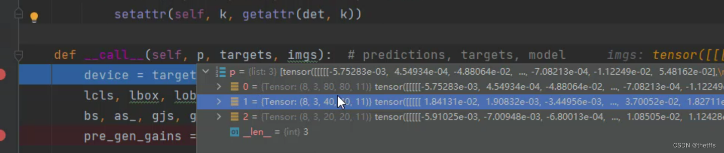
p传递的是3个输出层的预测值, (8,3,80,80,11)表示8个batch, 3个anchor, 特征图大小(80 * 80), 6分类对应的一个bbox向量维度是11。
标签targets
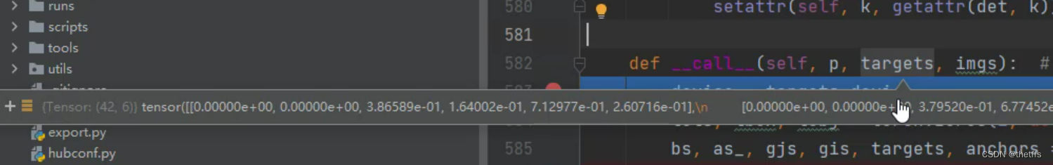
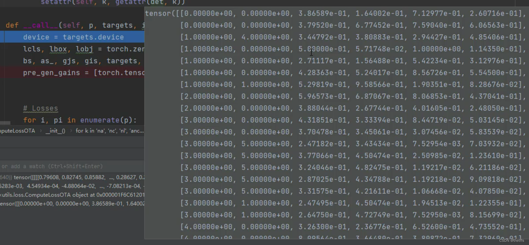
targets(42, 6) ,对应8batch的标注数据一共有42个,每个标注数据的信息用6维向量表示。分别是标签所在的batch id、标签的分类id、归一化的坐标框。
find_3_positive
find_3_positive实现了正样本分配策略。通过标注数据往左上或者右下偏移,能够增加正样本的数量。正样本对应的grid坐标和anchor id用来参与输出层的预测值计算。
  def find_3_positive(self, p, targets):
        # Build targets for compute_loss(), input targets(image,class,x,y,w,h)
        na, nt = self.na, targets.shape[0]  # number of anchors, targets
        indices, anch = [], []
        gain = torch.ones(7, device=targets.device).long()  # 7表示原标签6个+框ID(属于哪个大小的anchor)  normalized to gridspace gain
        ai = torch.arange(na, device=targets.device).float().view(na, 1).repeat(1, nt)  # same as .repeat_interleave(nt)
        targets = torch.cat((targets.repeat(na, 1, 1), ai[:, :, None]), 2)  # 就是最后加了一个维度,表示anchorID, append anchor indices

        g = 0.5  # bias 一会要玩漂移,
        off = torch.tensor([[0, 0],
                            [1, 0], [0, 1], [-1, 0], [0, -1],  # j,k,l,m
                            # [1, 1], [1, -1], [-1, 1], [-1, -1],  # jk,jm,lk,lm
                            ], device=targets.device).float() * g  # offsets

        for i in range(self.nl):#有3个输出层,分别做
            anchors = self.anchors[i]#当前输出层对应anchor
            gain[2:6] = torch.tensor(p[i].shape)[[3, 2, 3, 2]]  # 赋值,一会用,xyxy gain

            # Match targets to anchors,这块在遍历看看这些GT到底放在哪个的输出层合适
            t = targets * gain#归一化的标签映射到特征图上
            if nt:
                # Matches
                r = t[:, :, 4:6] / anchors[:, None]  # 每一个GT与anchor大宽高比大小,wh ratio
                j = torch.max(r, 1. / r).max(2)[0] < self.hyp['anchor_t']  # 0.25<比例<4才会被保留 compare
                # j = wh_iou(anchors, t[:, 4:6]) > model.hyp['iou_t']  # iou(3,n)=wh_iou(anchors(3,2), gwh(n,2))
                t = t[j]  # filter

                # Offsets
                gxy = t[:, 2:4]  # 到左上角的距离 grid xy
                gxi = gain[[2, 3]] - gxy  # 到右下角的距离 inverse
                j, k = ((gxy % 1. < g) & (gxy > 1.)).T#离左上角近的选出来,而且不能是边界
                l, m = ((gxi % 1. < g) & (gxi > 1.)).T#离右下角近的选出来,而且不能是边界
                j = torch.stack((torch.ones_like(j), j, k, l, m))#5个,因为自己所在实际位置一定为true
                t = t.repeat((5, 1, 1))[j]#相当于原来就1个 现在还要考虑2个邻居 target必然增多
                offsets = (torch.zeros_like(gxy)[None] + off[:, None])[j]#对应区域玩对应漂移大小 都是0.5个单位
            else:
                t = targets[0]
                offsets = 0

            # Define
            b, c = t[:, :2].long().T  # batch, class
            gxy = t[:, 2:4]  # grid xy
            gwh = t[:, 4:6]  # grid wh
            gij = (gxy - offsets).long()#漂移后 整数部分就是格子的索引
            gi, gj = gij.T  # grid xy indices

            # Append
            a = t[:, 6].long()  # 每一个target对应的anchor indices
            indices.append((b, a, gj.clamp_(0, gain[3] - 1), gi.clamp_(0, gain[2] - 1)))  # batch, anchor, grid indices
            anch.append(anchors[a])  # anchors大小

        return indices, anch
ai
已知模型有3个输出层,每个输出层有3个尺寸的anchor。对于targets我们初始化一个ai(3,42),用来表示targets和anchor可能存在的对应关系。
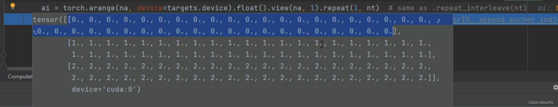
- torch.arange(na, device=targets.device):这个函数创建了一个从0到na(不包括na)的一维张量,其中na是一个整数。这个张量被创建在targets.device上,这意味着它会在targets张量所在的设备上(例如CPU或GPU)。
- .float():这个方法将上一步创建的张量转换为浮点数类型。这是因为torch.arange默认生成整数类型的张量,而.float()可以确保后续操作中数值的精度。
- .view(na, 1):.view()方法用于改变张量的形状而不改变其数据。在这里,它将一维张量重新塑形为一个na x 1的二维张量。每个元素都变成了一个单独的行。
- .repeat(1, nt):.repeat()方法用于沿着指定的维度重复张量。在这里,它将上一步得到的二维张量在第二维(列)上重复nt次。结果是一个na x nt的二维张量,其中每一行都是原始arange张量的副本。
targets增加anchor信息
这一步操作的目的就是为了把anchor id添加到 targets中,将targets张量维度从[42, 6]—> [3, 42 , 7]。
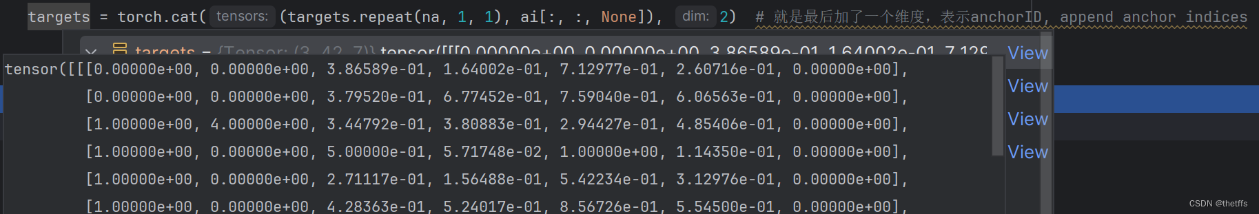
- targets.repeat(na, 1, 1):在第一个维度重复na边,第二和第三个维度保持不变 [42, 6]–>[3,42,6]
- ai[:, : , None] :该切片操作是在None的维度增加一维,但是元素的个数保持不变,用来扩充张量的维度,方便拼接。[3, 42, 1]
targets与anchor尺寸不匹配则滤掉
 # Matches
 r = t[:, :, 4:6] / anchors[:, None]  # 每一个GT与anchor大宽高比大小,wh ratio
 j = torch.max(r, 1. / r).max(2)[0] < self.hyp['anchor_t']  # 0.25<比例<4才会被保留 compare
 # j = wh_iou(anchors, t[:, 4:6]) > model.hyp['iou_t']  # iou(3,n)=wh_iou(anchors(3,2), gwh(n,2))
 t = t[j]  # filter
t[:, :, 4:6] 取标注数据的w和h与3个anchor的w和h做除法,大小不能超过4倍。过滤后匹配anchor大小的标注数据剩下39个。一个target可能对应多个anchor,所以过滤后的数据可能比开始的标注数据多。

计算offset是左上/右下
 # Offsets
                gxy = t[:, 2:4]  # 到左上角的距离 grid xy
                gxi = gain[[2, 3]] - gxy  # 到右下角的距离 inverse
                j, k = ((gxy % 1. < g) & (gxy > 1.)).T#离左上角近的选出来,而且不能是边界
                l, m = ((gxi % 1. < g) & (gxi > 1.)).T#离右下角近的选出来,而且不能是边界
                j = torch.stack((torch.ones_like(j), j, k, l, m))#5个,因为自己所在实际位置一定为true
                t = t.repeat((5, 1, 1))[j]#相当于原来就1个 现在还要考虑2个邻居 target必然增多
                offsets = (torch.zeros_like(gxy)[None] + off[:, None])[j]#对应区域玩对应漂移大小 都是0.5个单位
torch.stack()将多个张量按照新的维度进行堆叠。
计算新增样本grid索引
b, c = t[:, :2].long().T  # batch, class
            gxy = t[:, 2:4]  # grid xy
            gwh = t[:, 4:6]  # grid wh
            gij = (gxy - offsets).long()#漂移后 整数部分就是格子的索引
            gi, gj = gij.T  # grid xy indices
append新增正样本
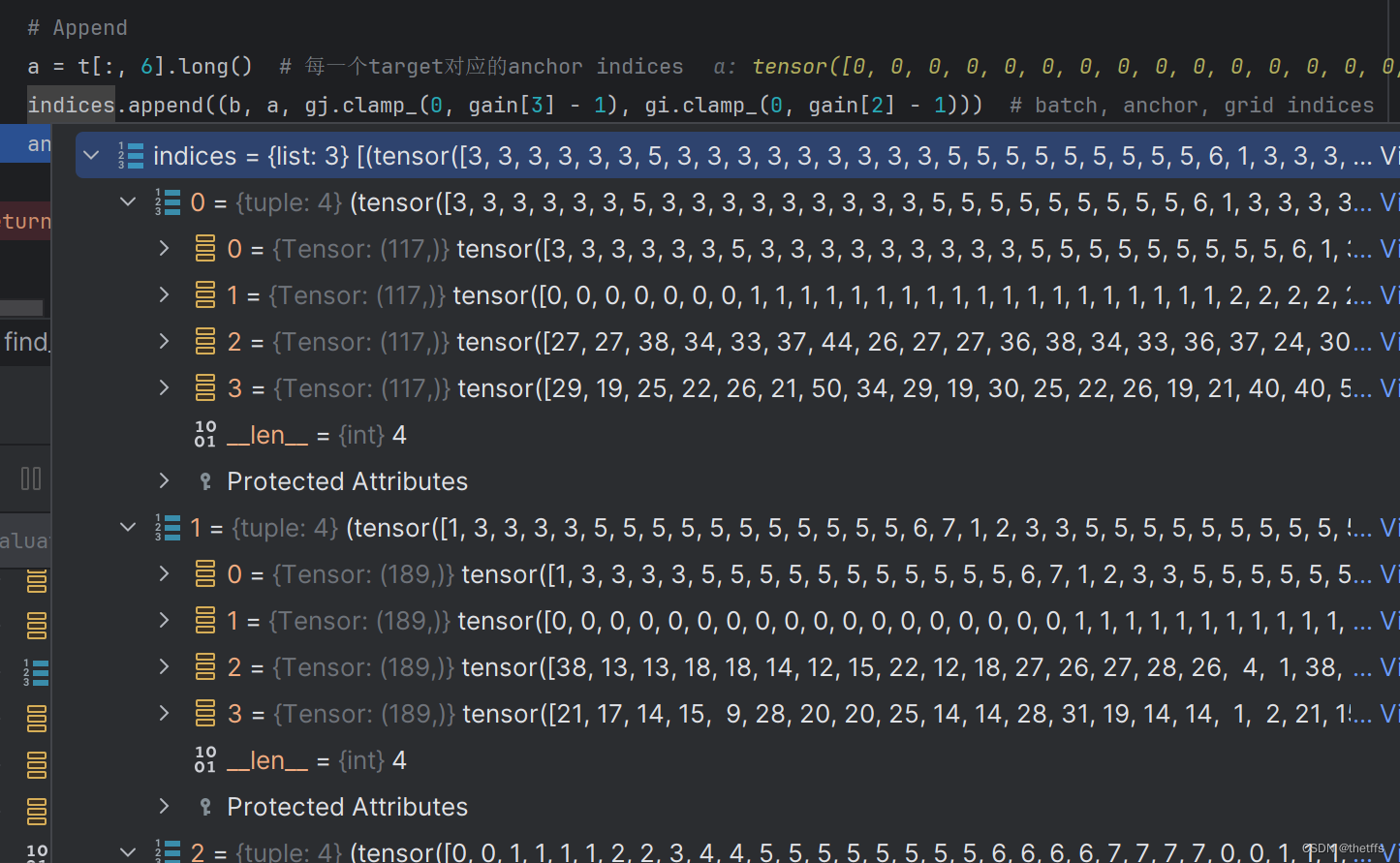
find_3_positive返回值
返回结果是anchor所在的grid的位置信息,以及是3个anchor中的anchor id。
build_target
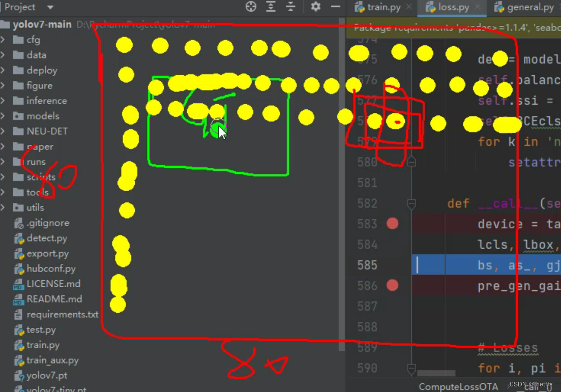
gt、grid、anchor
- 如下图所示黄色圆点表示grid,在特征图大小为80 * 80的输出层能用来预测目标框的grid的数量也有80 * 80个。
- 每个grid上有3个尺寸的anchor可以用,如图中3个叠加的红框所示。
- gt所在的grid用来生成预测值,不可能80 * 80个grid都用来预测目标框。gt所在的grid如何获取参考find_3_positive.
- gt 和 anchor尺寸超过4倍, 那么用来生成预测值的要素(gt、 grid、 anchor)会增加。 因此一个gt可能对应多个anchor。
候选框预测值的生成
经过函数find_3_position我们得到了更多的gt以及它的grid、anchor信息。这些信息和输出层输出的预测值需要搭配使用,这个步骤如下图所示(只看yolov7部分):
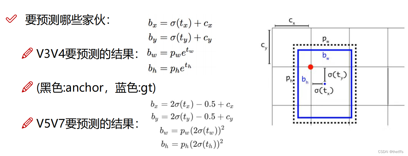
公式中的参数含义:
- tx, ty, tw, th(变量fg_pred ):这些值从模型输出层(变量pi)中索引得到的。索引即上文中计算得到的targets所在的grid坐标。我自己强行理解了这个grid坐标的作用:即target所在的gird本来就可以生成预测框,因此需要该grid在输出层中索引候选框的坐标。但是模型输出层不能一下输出正确的预测值,模型需要训练。因此使用上图公式,加上anchor的辅助计算能够得到更加合理的预测值。最后为了训练模型更新参数需要与标注数据计算LOSS。并且通过不断的迭代将LOSS降到最低。
- cx,cy(变量grid): 所在grid的坐标
- bx, by, bw, bh(变量pxywh ):目标的坐标框预测值,需要计算获得
- pw, ph(变量anch): 尺寸匹配的anchor的宽、高
fg_pred = pi[b, a, gj, gi]  #取对应target位置的预测结果
grid = torch.stack([gi, gj], dim=1)
pxy = (fg_pred[:, :2].sigmoid() * 2. - 0.5 + grid) * self.stride[i] #中心点在当前格子偏移量,-0.5到1.5之间 再还原 / 8.
pwh = (fg_pred[:, 2:4].sigmoid() * 2) ** 2 * anch[i][idx] * self.stride[i] #之前是考虑四倍,这也得同步  / 8.
pxywh = torch.cat([pxy, pwh], dim=-1)
pxyxy = xywh2xyxy(pxywh)
pair_wise_iou = box_iou(txyxy, pxyxy)#计算GT与所有候选正样本的IOU
pair_wise_iou_loss = -torch.log(pair_wise_iou + 1e-8)#IOU损失
build_targets
附源码:
def build_targets(self, p, targets, imgs):
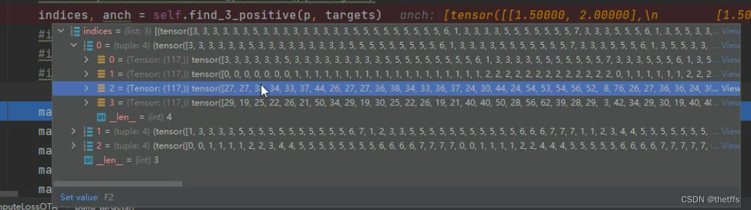
#indices, anch = self.find_positive(p, targets)
indices, anch = self.find_3_positive(p, targets)
#indices, anch = self.find_4_positive(p, targets)
#indices, anch = self.find_5_positive(p, targets)
#indices, anch = self.find_9_positive(p, targets)
matching_bs = [[] for pp in p]
matching_as = [[] for pp in p]
matching_gjs = [[] for pp in p]
matching_gis = [[] for pp in p]
matching_targets = [[] for pp in p]
matching_anchs = [[] for pp in p]
#p是list,每个list存放不同尺寸的预测头的预测值
# p[0]:[8,3,80,80,11]
# p[1]:[8,3,40,40,11]
# p[2]:[8,3,20,20,11]
nl = len(p)
for batch_idx in range(p[0].shape[0]):
# targets[42, 6]表示一个8batch的gt
b_idx = targets[:, 0]==batch_idx
#this_target表示输入当前图像的gt索引
#eg:this_target[2,6] 2表示有两个标注框,6表示标注框具体的值
this_target = targets[b_idx]#当前图像里的标注框GT
if this_target.shape[0] == 0:
continue
txywh = this_target[:, 2:6] * imgs[batch_idx].shape[1]#得到实际大小
txyxy = xywh2xyxy(txywh)
pxyxys = []
p_cls = []
p_obj = []
from_which_layer = []
all_b = []
all_a = []
all_gj = []
all_gi = []
all_anch = []
for i, pi in enumerate(p):#遍历每一个输出层
b, a, gj, gi = indices[i]
idx = (b == batch_idx)
b, a, gj, gi = b[idx], a[idx], gj[idx], gi[idx]
all_b.append(b)
all_a.append(a)
all_gj.append(gj)
all_gi.append(gi)
all_anch.append(anch[i][idx])
from_which_layer.append(torch.ones(size=(len(b),)) * i)#来自哪个输出层
fg_pred = pi[b, a, gj, gi] #取对应target位置的预测结果
p_obj.append(fg_pred[:, 4:5])
p_cls.append(fg_pred[:, 5:])
grid = torch.stack([gi, gj], dim=1)
pxy = (fg_pred[:, :2].sigmoid() * 2. - 0.5 + grid) * self.stride[i] #中心点在当前格子偏移量,-0.5到1.5之间 再还原 / 8.
#pxy = (fg_pred[:, :2].sigmoid() * 3. - 1. + grid) * self.stride[i]
pwh = (fg_pred[:, 2:4].sigmoid() * 2) ** 2 * anch[i][idx] * self.stride[i] #之前是考虑四倍,这也得同步 / 8.
pxywh = torch.cat([pxy, pwh], dim=-1)
pxyxy = xywh2xyxy(pxywh)
pxyxys.append(pxyxy)
pxyxys = torch.cat(pxyxys, dim=0)
if pxyxys.shape[0] == 0:
continue
p_obj = torch.cat(p_obj, dim=0)
p_cls = torch.cat(p_cls, dim=0)
from_which_layer = torch.cat(from_which_layer, dim=0)
all_b = torch.cat(all_b, dim=0)
all_a = torch.cat(all_a, dim=0)
all_gj = torch.cat(all_gj, dim=0)
all_gi = torch.cat(all_gi, dim=0)
all_anch = torch.cat(all_anch, dim=0)
#txyxy2各真实值 pxyxys:18个候选框
pair_wise_iou = box_iou(txyxy, pxyxys)#计算GT与所有候选正样本的IOU
pair_wise_iou_loss = -torch.log(pair_wise_iou + 1e-8)#IOU损失
top_k, _ = torch.topk(pair_wise_iou, min(10, pair_wise_iou.shape[1]), dim=1)#多的话选10个,少的话有几个算几个
dynamic_ks = torch.clamp(top_k.sum(1).int(), min=1)#累加,相当于有些可能太小的我不需要,宁缺毋滥?
#gt_cls_per_image[2,18,6]含义:18个候选框,2个gt,6分类,每个候选框对于每个gt,它的分类是什么
gt_cls_per_image = (
F.one_hot(this_target[:, 1].to(torch.int64), self.nc)
.float()
.unsqueeze(1)
.repeat(1, pxyxys.shape[0], 1)#onehot后重复候选框数量次
)
num_gt = this_target.shape[0]
# p_obj 目标置信度,预测类别的时候做了个加权,即是个目标物体的前提,预测你的类别是什么
cls_preds_ = (
p_cls.float().unsqueeze(0).repeat(num_gt, 1, 1).sigmoid_()
* p_obj.unsqueeze(0).repeat(num_gt, 1, 1).sigmoid_()
)#预测类别情况
#把类别的真实值和预测值传进去做交叉熵损失函数
y = cls_preds_.sqrt_()
pair_wise_cls_loss = F.binary_cross_entropy_with_logits(
torch.log(y/(1-y)) , gt_cls_per_image, reduction="none"
).sum(-1)#类别差异
del cls_preds_
#候选框复筛,考虑IOU损失和类别损失的加权影响
cost = (
pair_wise_cls_loss
+ 3.0 * pair_wise_iou_loss
)#候选框里要开始选了,要看他们的IOU情况和分类情况 综合考虑
matching_matrix = torch.zeros_like(cost)
for gt_idx in range(num_gt):
_, pos_idx = torch.topk(
cost[gt_idx], k=dynamic_ks[gt_idx].item(), largest=False
)
matching_matrix[gt_idx][pos_idx] = 1.0
del top_k, dynamic_ks
anchor_matching_gt = matching_matrix.sum(0)#竖着加
if (anchor_matching_gt > 1).sum() > 0:#一个正样本匹配到了多个GT的情况
_, cost_argmin = torch.min(cost[:, anchor_matching_gt > 1], dim=0)#那就比较跟哪个一个损失最小,删除其他
matching_matrix[:, anchor_matching_gt > 1] *= 0.0#其他删除
matching_matrix[cost_argmin, anchor_matching_gt > 1] = 1.0#最小的那个保留
fg_mask_inboxes = matching_matrix.sum(0) > 0.0#哪些是正样本
matched_gt_inds = matching_matrix[:, fg_mask_inboxes].argmax(0)#每个正样本对应的真实框索引
from_which_layer = from_which_layer[fg_mask_inboxes]
#from_which_layer = from_which_layer.to(fg_mask_inboxes.device)
all_b = all_b[fg_mask_inboxes]#对应的batch索引
all_a = all_a[fg_mask_inboxes]#对应的anchor索引
all_gj = all_gj[fg_mask_inboxes]
all_gi = all_gi[fg_mask_inboxes]
all_anch = all_anch[fg_mask_inboxes]
this_target = this_target[matched_gt_inds]#匹配到正样本的GT
for i in range(nl):#得到每一层的正样本
layer_idx = from_which_layer == i
matching_bs[i].append(all_b[layer_idx])
matching_as[i].append(all_a[layer_idx])
matching_gjs[i].append(all_gj[layer_idx])
matching_gis[i].append(all_gi[layer_idx])
matching_targets[i].append(this_target[layer_idx])
matching_anchs[i].append(all_anch[layer_idx])
for i in range(nl):#合并
if matching_targets[i] != []:
matching_bs[i] = torch.cat(matching_bs[i], dim=0)
matching_as[i] = torch.cat(matching_as[i], dim=0)
matching_gjs[i] = torch.cat(matching_gjs[i], dim=0)
matching_gis[i] = torch.cat(matching_gis[i], dim=0)
matching_targets[i] = torch.cat(matching_targets[i], dim=0)
matching_anchs[i] = torch.cat(matching_anchs[i], dim=0)
else:
matching_bs[i] = torch.tensor([], device='cuda:0', dtype=torch.int64)
matching_as[i] = torch.tensor([], device='cuda:0', dtype=torch.int64)
matching_gjs[i] = torch.tensor([], device='cuda:0', dtype=torch.int64)
matching_gis[i] = torch.tensor([], device='cuda:0', dtype=torch.int64)
matching_targets[i] = torch.tensor([], device='cuda:0', dtype=torch.int64)
matching_anchs[i] = torch.tensor([], device='cuda:0', dtype=torch.int64)
return matching_bs, matching_as, matching_gjs, matching_gis, matching_targets, matching_anchs
损失函数计算
iou损失
pair_wise_iou_loss = -torch.log(pair_wise_iou + 1e-8)#IOU损失
分类损失
fg_pred = pi[b, a, gj, gi]  #取对应target位置的预测结果
p_cls.append(fg_pred[:, 5:])
num_gt = this_target.shape[0]
cls_preds_ = (
    p_cls.float().unsqueeze(0).repeat(num_gt, 1, 1).sigmoid_()
    * p_obj.unsqueeze(0).repeat(num_gt, 1, 1).sigmoid_()
)#预测类别情况
 y = cls_preds_.sqrt_()
 pair_wise_cls_loss = F.binary_cross_entropy_with_logits(
    torch.log(y/(1-y)) , gt_cls_per_image, reduction="none"
 ).sum(-1)#类别差异
损失加权
cost = (
        pair_wise_cls_loss
         + 3.0 * pair_wise_iou_loss
     )#候选框里要开始选了,要看他们的IOU情况和分类情况 综合考虑
总结
本文主要目的是为了梳理yolov7输出层预测的目标框坐标的整个过程。